This article is part of a set of three; the common factor is Calculus of Variations. In classical physics Calculus of Variations is applied in three areas: Optics, Statics, and Dynamics. Discussion of application in statics is included in the 'Foundation' article.
The other two articles:

Foundation:	Calculus of Variations
Optics:	Fermat's stationary time

I strongly recommend to first absorb the contents of the 'Calculus of Variations' article.

The Energy-Position equation

1. From F = ma to the Work-Energy theorem

2. From Work-Energy to stationary action

3. Trial trajectories: response to variation
    3.1 Potential increases linear with height
    3.2 Potential increases quadratic with displacement
    3.3 Potential increases proportional to cube of displacement

Appendix I The meaning of stationary

Appendix II Jacob's Lemma

This exposition is about Hamilton's stationary action. The usual presentation is to posit Hamilton's stationary action, and to proceed with showing that F = ma can be recovered from it. However, it is also possible to proceed in the other direction. You can start with F = ma, and proceed to Hamilton's stationary action in all forward steps. The development is in two stages:
- Derivation of the Work-Energy theorem from F = ma
- Demonstration that in cases where the Work-Energy theorem holds good Hamilton's stationary action will hold good also.

The Work-Energy theorem and Hamilton's stationary action have the following in common: the physics taking place is described in terms of kinetic energy and potential energy. As an overarching name for both the Work-Energy theorem and Hamilton's stationary action I will use the expression 'energy mechanics'.

Interactive diagrams
The intention of this article is to let the interactive diagrams tell the story. You can choose to jump ahead to the interactive diagrams However, I strongly recommend you return to these paragraphs at some point; for overall understanding they are necessary.

Requirement for well defined potential energy

Given a particular force: in order to have a well defined expression for potential energy the force must have the property that the work done in moving from some point A to some point B is independent of the path taken between the two points. The validity of energy mechanics is limited to forces with that property.

(It may be that in terms of a deeper theory such as quantum physics all interactions actually have that potential-is-independent-of-the-path property, but we should not blindly assume that.)

As we know: the principle of conservation of energy is asserted without any restriction. That's why the concept is referred as a 'principle', it is a blanket statement.

The discussion in this article avoids the blanket statement. The discussion in this article is limited to the classes of cases where by way of experimental corroboration it is evident that the work done in moving from some point A to some point B is independent of the path taken between the two points.

1. From F = ma to the Work-Energy theorem

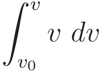
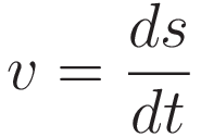
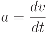
In preparation for deriving the work-energy theorem we first derive a kinematical relation between the integral of acceleration with respect to position, and velocity.

In the course of the derivation the following two relations will be used:

$ds = v \ dt$

(1.1)

$dv = a \ dt$

(1.2)

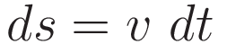
Let a represent an arbitrary acceleration profile. We set up integration of this acceleration profile from a starting point s₀ to a final point s

$\int_{s_0}^s a \ ds$

(1.3)

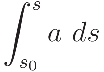
Intermediary step: change of the differential according to (1.1), with corresponding change of limits.

$\int_{t_0}^t a \ v \ dt$

(1.4)

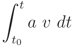
Change the order:

$\int_{t_0}^t v \ a \ dt$

(1.5)

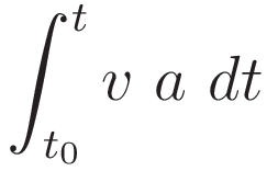
Change of the differential according to (1.2), with corresponding change of limits.

$\int_{v_0}^v v \ dv$

(1.6)

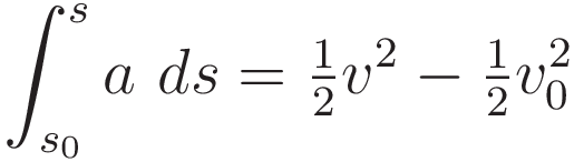
So we have:

$\int_{s_0}^s a \ ds = \tfrac{1}{2}v^2 - \tfrac{1}{2}v_0^2$

(1.7

I want to emphasize just how general the validity of (1.7) is: it follows from the definitions (1.1) and (1.2) and the mathematics of differentiation/integration. That is: (1.7) obtains mathematically, independent from any physics.

The Work-Energy theorem

We start with the force-acceleration principle:

(1.8)

Specify integration with respect to the position coordinate:

$\int_{s_0}^s F \ ds = \int_{s_0}^s ma \ ds$

(1.9)

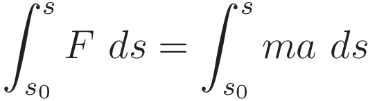
Use (1.7) to process the right hand side. The result is the work-energy theorem:

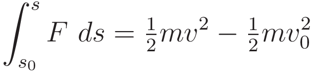
$\int_{s_0}^s F \ ds = \tfrac{1}{2}mv^2 - \tfrac{1}{2}mv_0^2$

(1.10)

The work-energy theorem motivates the definitions of potential energy and kinetic energy.

Historically: for several centuries, from the time of Huygens to the time of Hamilton, the concept of 'living force' was used, which was defined as mv². It was in the 1850's that the physics community shifted to a new name and a new definition: ½mv². The benefit of that shift: by defining kinetic energy as an integral (integral of ma with respect to the position coordinate) the concept of kinetic energy is defined in terms of the work-energy theorem.

To emphasize the structure of the Work-Energy theorem I give the elements arranged in a table. In each row the statement follows mathematically from the statements in the row(s) above it.

	$v = \frac{ds}{dt}$	$a = \frac{dv}{dt}$
	$\int_{s_0}^s a \ ds = \tfrac{1}{2}v^2 - \tfrac{1}{2}v_0^2$
$\int_{s_0}^s F \ ds = \tfrac{1}{2}mv^2 - \tfrac{1}{2}mv_0^2$

Potential energy

Historically the concept of potential energy arose before the work-energy theorem reached today's standard form. With the benefit of hindsight we recognize that the concept of potential energy capitalizes on the work-energy theorem.

Potential energy is defined as the negative of the left hand side of (1.9); the integral of force over distance.

$\Delta E_p = - \int_{s_0}^s F \ ds$

(1.10)

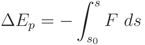
In order for the potential energy to be well defined a specific condition must be met: the value of the integral from point s₀ to point s must be independent of how the test object moves from point s₀ to point s.

When the potential energy is well defined:

$\Delta (E_k) = - \Delta (E_p)$

(1.11)

That is: with potential energy defined according to (1.10): when an object is moving down a potential gradient the kinetic energy will increase by the amount that the potential energy decreases. (With everything reversed when moving in the opposite direction, of course.)

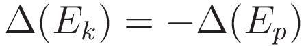
(1.12) combines three statements. I present these three statements as a unit to emphasize the interconnection between them. While the statements are different mathematically, the physics content of these three is the same.

$\begin{array}{rcl} F & = & ma \\[+10pt] \int_{s_0}^s F \ ds & = & \tfrac{1}{2}mv^2 - \tfrac{1}{2}mv_0^2 \\[+10pt] -\Delta E_p & = & \Delta E_k \end{array}$

(1.12)

2. From Work-Energy to stationary action

2.1 Preparation: discussion of notation of Hamilton's stationary action and of the Euler-Lagrange equation.

Graphlet 2.1 sets out how in the diagrams on this pages the variation is implemented. The grey line represents a true trajectory. The trial trajectory is obtained by multiplying the true trajectory with a factor, here the multiplication factor is the slider value

Picture 2.1 Graphlet
Application of variation

In graphlet 2.1 a single slider has been implemented. That means that for the representation in graphlet 2.1 the variation space is a 1-dimensional space: the value of the slider. The graphlets in section 3 have multiple sliders, for granular control.

In preparation:
Hamilton's stationary action and dimensional analysis

In equation (2.1) the differention that is stated is differentiation with respect to the variation sweep as presented in graphlet 2.1

In the notation the greek lowercase $ \delta $ is used to signal a difference: the expression that is differentiated states an integral.

\[ \frac {\delta ( \ \int_{t_1}^{t_2} (E_k - E_p)\ dt \ )}{\delta s} = 0 \]

(2.1)

The general form for the Euler-Lagrange differential operator, For a lagrangian $L$

\[ \frac{\partial L}{\partial s} - \frac{d}{dt}\left( \frac{\partial L}{\partial v} \right) \]

(2.2)

With the Lagrangian $ (E_k-E_p) $ inserted in the Euler-Lagrange operator we get:

\[ \frac{\partial (E_k-E_p)}{\partial s} - \frac{1}{dt}\left( \frac{\partial (E_k-E_p)}{\partial v} \right) = 0 \]

(2.3)

We have the following properties:

$\tfrac{\partial E_k}{\partial s} = 0$, $\tfrac{\partial E_p}{\partial v} = 0$, $\tfrac{\partial E_p}{\partial s} = \tfrac{d E_p}{d s}$ and $\tfrac{\partial E_k}{\partial v} = \tfrac{d E_k}{dv} $

Therefore:

$\frac{\partial (E_k-E_p)}{\partial s} = \frac{d(-E_p)}{ds} $

And:

$\frac{1}{dt}\frac{\partial (E_k-E_p)}{\partial v} = \frac{d}{dt}( \frac{dE_k}{dv}) $

So (2.3) simplifies to the expression below:

\[ \frac{d(-E_p)}{ds} - \frac{d}{dt} \left( \frac{dE_k}{dv} \right) = 0 \]

(2.4)

It looks as if the differential operation performed on the $E_k$ term is different from the operation performed on the $E_p$ term, but that is not actually the case.

For one thing: in order for (2.4) as a whole to be self-consistent the differential operation that is performed on the $E_k$ term must be dimensionally the same as the operation performed on the $E_p$ term

In (2.5) the dimensionality of (2.4) is made explicit by stating the velocity coordinate $v$ in the form $\tfrac{ds}{dt}$

\[ \frac{d(-E_p)}{ds} - \frac{d}{dt} \left( \frac{dE_k}{d(\frac{ds}{dt})} \right) = 0 \]

(2.5)

\[ \frac{d(-E_p)}{ds} - \frac{d}{\cancel{dt}} \left( \frac{dE_k}{d(\frac{ds}{\cancel{dt}})} \right) = 0 \]

(2.6)

In (2.6): dimensionally the two occurences of $dt$ drop out of the differentiation. Further down we will return to this.

From the work-energy theorem to the Lagrange equation

We start with repeating (1.10), the work-energy theorem:

\[ \int_{s_0}^s F \ ds = \tfrac{1}{2}mv^2 - \tfrac{1}{2}mv_0^2 \]

(2.7)

The next step: differentiate both sides with respect to the position coordinate $s$:

\[ \frac{d(\int_{s_0}^s F \ ds)}{ds} = \frac{d(\tfrac{1}{2}mv^2)}{ds} \]

(2.8)

We know in advance that (2.8) will recover $F=ma$; we saw in the derivation of the work-energy theorem that integration of $ma$ with respect to position coordinate $s$ gives $\tfrac{1}{2}mv^2$; the differentiation will recover $ma$.

For the quantity $\tfrac{1}{2}mv^2$ the following two differentiation operations are the same:

\[ \frac{d(\tfrac{1}{2}mv^2)}{ds} \ \Leftrightarrow \ \frac{d}{dt}\frac{d (\tfrac{1}{2}mv^2)}{d v} \]

(2.9)

This was hinted at with (2.6), the two operations are dimensionally the same.

In this context the circumstance that allows the two to be fully the same is that position, velocity, and acceleration are related by differentiation; velocity is itself defined as a differential relation.

(2.8) rearranges into the following form:

\[ \frac{d(-E_p)}{ds} - \frac{d}{dt} \left( \frac{dE_k}{dv} \right) = 0 \]

(2.10)

(2.10) shows: inserting the Lagrangian $ (E_k-E_p) $ into the Euler-Lagrange differential operator gives an expression that differentiates the energy with respect to position coordinate

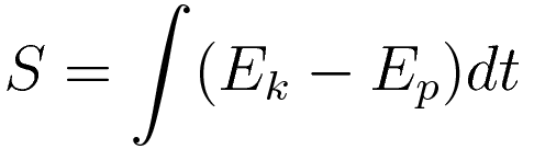
I will refer to the form of (2.8) as 'the energy-position equation'; the energy is differentiated with respect to position coordinate.

The remaining step is to go from the energy-position equation to Hamilton's stationary action

In the interactive diagram below: in the second panel Force and acceleration are represented. For simplicity the value of the mass $m$ is set to one, so that the values of the Force and the acceleration are the same

Picture 2.2. Graphlet

As you sweep out variation: the true trajectory has the property that the acceleration is equal to the force $F$.

The case presented in the diagram is of a potential that increases with the cube of the height. Close to height zero the force is very small, so in that region there is hardly any change in the slope of the trajectory. As the object climbs the force rapidly increases, and there is a rapid turnaround.

Green bars: the magnitude of the accelerating force.
Red bars: the magnitude of the acceleration caused by the force.

With the two checkboxes you can switch the visibility of the red bars and green bars. As you sweep out variation: the response of the red bars to variation is in linear proportion. Example: when you make the trial trajectory half the height of the true trajectory the red bars are half the height. The reason why the red bars response is in linear proportion: when you make the trial trajectory half as high the slope is half as steep, resulting in half the acceleration.

In this diagram the green bars respond in quadratic proportion to the variation. In the case represented here the potential is proportional to the cube of the height. Hence the force is proportional to the square of the height.

The force and the acceleration respond differently to applying variation; that is why there is only a single point in variation space where the two values are the same.

Next we define a differentiation with a notation of its own: differentiation of energy with respect to applied variation. The general convention is to use the greek undercase $\delta$ to signal that the differentiation is differentiation with resepct to variation.

\[ \frac{\delta E_k}{\delta s} = \frac{\delta E_p}{\delta s} \]

(2.11)

The applied variation isn't a physical motion. The applied variation is a hypothetical change for the purpose of getting a differentiation out of it.

In the case of physical motion the kinetic energy and potential energy are counter-changing: the sum of the two energies is a conserved quantity. The differentiation with respect to position coordinate inherits that property:

\[ \frac{d E_k}{d s} + \frac{dE_p}{d s} = 0 \]

(2.12)

But when differentiating with respect to variation the changes of the two energies are co-directional. When two quantities are changing co-directionally then in order two see when they are the same you must subtract one from the other:

\[ \frac{\delta E_k}{\delta s} - \frac{\delta E_p}{\delta s} = 0 \]

(2.13)

(2.12) and (2.13) are not the same differentiation. (2.12) is for the case of physical motion, (2.13) is for the case of virtual change. The connection is that the differentiations have the same ratio: at the point in variation space where the trial trajectory coincides with the true trajectory (2.12) and (2.13) both are satisfied; each is sufficient to imply the other.

We now have the means in place to go from the energy-position equation (2.8) to Hamilton's stationary action.

The true trajectory has the property that continuously through time the acceleration matches the force.

In graphlet 2.2: the set of all red bars covers a surface area, and the set of all green bars covers a surface area. We can set up the following demand: for any pair of time coordinates $t_1$ and $t_2$ the following relation must be satisfied:

\[ \int_{t_1}^{t_2} \lvert F \rvert \ dt = \int_{t_1}^{t_2} \lvert ma \rvert \ dt \]

(2.14)

Note especially: this is not for a particular choice of $t_1$ and $t_2$. This is the demand: within the domain: for the combination of any value of $t_1$ and any value of $t_2$ the relation must be satisfied.

Substitute: $ \lvert F \rvert \ \Leftrightarrow \tfrac {\delta E_p}{\delta s} $ and $ \lvert ma \rvert \ \Leftrightarrow \tfrac {\delta E_k}{\delta s} $ :

\[ \int_{t_1}^{t_2} \left( \frac {\delta E_p}{\delta s} \right) dt = \int_{t_1}^{t_2} \left( \frac {\delta E_k}{\delta s} \right) dt \]

(2.15)

Bring the two terms to the same side:

\[ \int_{t_1}^{t_2} \left( \frac {\delta E_k}{\delta s} \right) dt - \int_{t_1}^{t_2} \left( \frac {\delta E_p}{\delta s} \right) dt = 0 \]

(2.16)

Combine the integrations:

\[ \int_{t_1}^{t_2} \left( \frac {\delta E_k}{\delta s} - \frac {\delta E_p}{\delta s} \right) dt = 0 \]

(2.17)

combine the differentiations:

\[ \int_{t_1}^{t_2} \left( \frac {\delta (E_k - E_p)}{\delta s} \right) dt =0 \]

(2.18)

The following equivalence expresses a key transition.

The circumstance underlying the equivalence is this combination of properties:
- the applied variation is variation of position coordinate
- the integration is integration with respect to time.
Those two operations are independent: they don't affect each other. Because of that: changing the order of the operations doesn't change the outcome:

\[ \int_{t_1}^{t_2} \left( \frac {\delta (E_k - E_p)}{\delta s} \right) dt \quad \Leftrightarrow \quad \frac {\delta \left( \int_{t_1}^{t_2} (E_k - E_p)\ dt \right)}{\delta s} \]

(2.19)

Given the equivalence expressed in (2.19): (2.18) can be restated in the form below:
The form below is the same as (2.1). It is Hamilton's stationary action.

\[ \frac {\delta ( \ \int_{t_1}^{t_2} (E_k - E_p)\ dt \ )}{\delta s} = 0 \]

(2.20)

3. Trial trajectories: response to variation

The following three graphlets are three instances of the same graphlet, for three successive classes of cases.

As you manipulate the sliders: the process to home in on the true trajectory is to manipulate the trial worldline such that over the entire trajectory the slope of the kinetic energy curve (red) matches the slope of the potential energy curve (green). When the trial trajectory is at thet the point in variation space such that those two slopes match the derivative of Hamilton's action is zero.

3.1 Potential increases linear with height

Picture 3.1. Graphlet
Potential energy increases linear with height; the trajectory is a parabola

Graphlet 3.1 is for the case of a uniform force, causing an acceleration of 2 m/s².
As we know: with a uniform force the curve that represents the height as a function of time is a parabola.

In the 'energy' sub-panel the green curve represents the minus potential energy. In effect the potential energy curve has been flipped upside down. That way you can see directly that when the trial trajectory coincides with the true trajectory the red and green curve are parallel to each other everywhere.

(Any form of calculating the true trajectory uses the derivative of the potential energy. That is, in calculation the value of the potential energy itself is not used. Because of that the choice of zero point of potential energy is arbitrary.)

In the lower right subpanel:
The blue dot represents Hamilton's action.
The label of the horizontal axis is p_v, which stands for 'variational parameter'. The positioning of the dots corresponds to the value of the main slider.

In the case of linear potential: when the trial trajectory coincides with the true trajectory the value of Hamilton's action is minimal/minimized. In the case implemented in this graphlet: any change of the trial trajectory results in raising the value of Hamilton's action.

3.2 Potential increases quadratic with displacement

Picture 3.2. Graphlet
Potential energy increases quadratic with displacement

Graphlet 3.2 is for the case where the force increases in linear proportion to the displacement. This case is commonly referred to as Hooke's law.
As we know: With Hooke's law the resulting motion is harmonic oscillation and the curve that represents the displacement as a function of time is the sine function.

With Hooke's law the potential energy increases with the square of the displacement. That is: with Hooke's law we have that the rate of change of potential energy is on par with that of the kinetic energy: with Hooke's law the expressions for the energies are both quadratic expressions.

As we know: with Hooke's law the amplitude and period of the resulting oscillation are independent from each other. Hamilton's stationary action corroborates that: when the trial trajectory is the harmonic oscillation function then if you change the amplitude the value of the action remains the same.

(In the diagram the actual curve is the cosine function; the point is that it is the harmonic oscillation function.)

3.3 Potential increases proportional to cube of displacement

Picture 3.3. Graphlet
Potential energy proportional to cube of displacement.

Graphlet 3.3 is for the case where the force increases proportional to the square of the displacement, hence the potential energy increases with the cube.

Click the button 'Show numerical' to show how the curve displayed in graphlet 6 was independently verified

Comparing the trajectories

In graphlet 3.1 the potential energy as a function of position is linear. Whenever the potential energy as a function of position is of lower order than the expression for the kinetic energy the action reaches a minimum when the derivative of the action is zero. In graphlet 3.2 the potential energy function and the kinetic energy function are both quadratic expressions, so the action is neither a minimum nor a maximum. Here in graphlet 3.3 the potential energy as a function of position is a higher order expression than the one for the kinetic energy (cubic versus quadratic), and consequently when the derivative of the action is zero the action reaches a maximum.

I recommend enlarging the graphlet to the full width of the browser window. Visibility of the navigation column of this page can be toggled. When the navigation column has been hidden: use the button 'Larger' and zoom in on the page as a whole to make the graphlet fill the entire width of the browser window.

How to operate the demonstration:

The graphlet set 3.1, 3.2, and 3.3 is designed to be discoverable, but for the sake of completeness I provide a description.

The main slider, located at the bottom of the graphlet, executes a global variation sweep. The value displayed in the "knob" of the main slider is a value to implement the variation, from here on I will refer to it as the 'variational parameter p_v' In the 'integral' panel the variational parameter p_v is along the horizontal axis.

Names for the 4 sub-panels:
- upper left: Control panel
- lower left: Height panel
- upper right: Energies panel
- lower right: Integrals panel

Note: The 3 sub-panels with a coordinate system are named after their vertical axis name: Height, Energy, Integral.

In the starting configuration the trajectory points (height panel) have been placed such that they coincide (to a very good approximation) with the true trajectory of the object.

When the object is moving along the true trajectory the rate of change of kinetic energy matches the rate of change of potential energy (work-energy theorem). This match of rate of change has been emphasized by turning the graph of the potential energy (green) upside down. When the object is moving along the true trajectory the red and green curve have the same slope along the entire trajectory.

The energies panel is where it happens. The energies panel represents how the equation that you are using solves for the true trajectory.

Hamilton's Action

$S = \int (E_k - E_p) dt$

Hamilton's Action is represented by the blue dot in the Integrals panel. Use the main slider to sweep out variation. The blue dot follows a curve; it is a curve in variation space. The slope of that curve represents the derivative of Hamilton's Action with respect to variation.

At the point where over the entire trajectory the derivative of the kinetic energy is equal to the derivative of the minus potential energy the derivative of the blue dot is zero.

In the control panel the two sliders on the far left are adjusters for the trajectory. The upper adjuster morphs the trajectory towards a curve that is more blunt than the true trajectory; the lower adjuster morphs the trajectory towards a triangle shape.

These adjusters allow morphing of the trial trajectory while maintaining that during the entire ascent the velocity never reverses from decreasing to increasing again, which would be unphysical.

The row of ten sliders is for adjustment of individual nodes. The three radio buttons toggle between three sets of node adjusting sliders.
The '× 1' button: for a ratio of 1-to-1 of moving the slider and movement of the corresponding node of the trajectory.
The '× 0.1' button: ratio of 10 to 1
The '× 0.01' button: ratio of 100 to 1, for fine adjustment.

The button 'Consolidate':
Clicking the button 'Consolidate' does the following: the current value of the '× 0.1' slider is transferred to the '× 1' slider. That is: after clicking the button 'Consolidate' the position of the '× 0.1' slider is reset to its zero position, and the '× 1' slider has been incremented accordingly.

In the energies panel: the grey point is draggable, and it drags the entire curve of the kinetic energy (red) with it. By shifting the kinetic energy curve over to the potential energy curve the user can verify that the red and green curve are parallel to each other along the entire trajectory. (The evaluation of the integral uses the unshifted position of the kinetic energy curve.)

In the integrals panel:
· Red/Green point: value of the integral of the red/green curve of the energies panel
· Blue point: the sum of the values of the red point and the green point

Finding the true trajectory by adjusting the sliders

As a seed move the '× 1' sliders so that the nodes are positioned along a straight line, say at 45 degrees.
In the 'Energies' subpanel, move the graph of the kinetic energy (red dots) down, on average a bit below the potential energy graph (green dots)
Use the '× 0.1' sliders to move the nodes upward bringing the red dots and green dots into alignment.
The true trajectory has the property that the rate of change of kinetic energy matches the rate of change of potential energy, so you want to make those two curves parallel to each other.

Picture I.1. Graphlet
Infinitesimal variation δs

Appendix I: The meaning of 'stationary'

Picture II.1. Graphlet
At the x-coordinate where the red and green curve have equal slope the blue curve is at zero slope.

Red and green are both ascending functions. We want to identify the coordinate where the rate of change of the red value matches the rate of change of the green value. The shortest way to get there is by setting up an equation with the derivative of the red curve on one side and the derivative of the green curve on the other side.

$\frac{d\left( \ f(x) \ \right)}{dx} = \frac{d \left( \ g(x) \ \right)}{dx}$

(I.1)

$\frac{d(\tfrac{1}{2}x^2)}{dx} = \frac{d(ln(x)-\tfrac{1}{2})}{dx}$

(I.2)

$x = \frac{1}{x}$

(I.3)

In the case of Hamilton's stationary action the same comparison is performed, but in a form that takes more steps. We see the following: a third function is defined, which is called the Lagrangian L: L=(E_k-E_p), and the point to be identified is called the point of 'stationary action'. 'Stationary action' is another way of saying: identify the point where the derivative of the Lagrangian is zero.

Summerizing:
Hamilton's stationary action works by imposing the constraint that was established with (1.11): the rate of change of kinetic energy must match the rate of change of potential energy.

Appendix II: Jacob's Lemma

When Johann Bernoulli had presented the Brachistochrone problem to the mathematicians of the time Jacob Bernoulli was among the few who was able to find the solution independently. The treatment by Jacob Bernoulli is in the Acta Eruditorum, May 1697, pp. 211-217

Jacob opens his treatment with an observation concerning the fact that the curve that is sought is a minimum curve.

Picture II.1. Image
Jacob's Lemma

Image source:
Acta Eruditorum 1697 p. 205

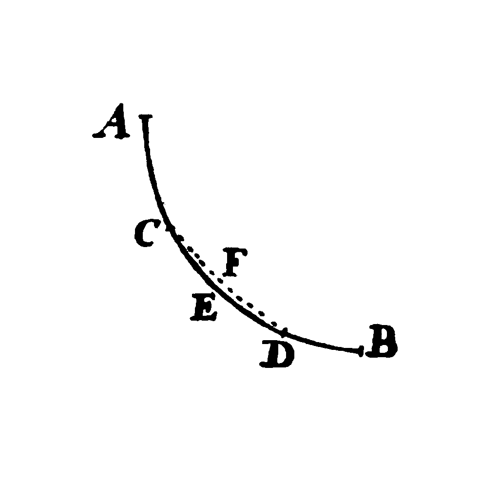
Lemma. Let ACEDB be the desired curve along which a heavy point falls from A to B in the shortest time, and let C and D be two points on it as close together as we like. Then the segment of arc CED is among all segments of arc with C and D as end points the segment that a heavy point falling from A traverses in the shortest time. Indeed, if another segment of arc CFD were traversed in a shorter time, then the point would move along ACFDB in a shorter time than along ACEDB, which is contrary to our supposition.

Jacob's lemma generalizes to all cases where the curve that you want to find is an extremum; either a maximum or a minimum. If the evaluation is an extremum for the entire curve, then it is also an extremum for any sub-section of the curve, down to infinitesimally short subsections.

The interactive diagrams on this page are created with the Javascript Library JSXGraph. JSXGraph is developed at the Lehrstuhl für Mathematik und ihre Didaktik, University of Bayreuth, Germany.

This work is licensed under a Creative Commons Attribution-ShareAlike 3.0 Unported License.