This article is part of a set of three; the common factor is Calculus of Variations. In classical physics Calculus of Variations is applied in three areas: Optics, Statics, and Dynamics. Discussion of application in statics is included in the 'Foundation' article.
The other two articles:
| Foundation: | Calculus of Variations |
| Dynamics: | Energy Position Equation |
Fermat's stationary time
Refraction
When light transitions from one medium to another there is refraction. This refraction is described by Snell's law. Snell's law is inferred from the experimental data.
Christiaan Huygens proposed a way of understanding Snell's law in terms of reconstitution of a wavefront. It is common to refer to this idea as ‘Huygens' Principle’. I actually prefer to use the designation ‘wavefront hypothesis’.
(In my opinion the qualification ‘Principle’ is used too often. If everything is a principle then the word ‘principle’ is rendered meaningless.)
It is assumed that the wavefront is always perpendicular to the direction of propagation.
Refraction by wavefront reconstitution
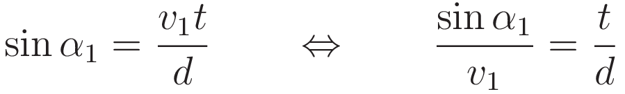

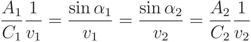
(3) follows from (1) and (2). (3) is a way of stating Snell's law:
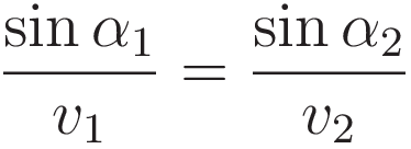
Image 1. shows how Huygens' wavefront hypothesis gives Snell's law
The next stage is to show how Huygens' wavefront hypothesis is sufficient to imply Fermat's stationary time.
Time and Space
We can express the length of the path that light takes in terms of spatial length, or in terms of duration, the interconversion is straightforward.
Huygens' wavefront hypothesis and Fermat's stationary time have as common factor the supposition that in an optically denser medium light propagates slower. Huygens' wavefront hypothesis has the additional supposition that the propagation has a wave character.
Incidentally, according to the wavefront hypothesis the frequency of the propagating wave remains the same. So the process of refraction can be seen as a process that conserves the frequency of the propagating wave.
Right-angled triangles
To set things up for discussing Fermat's stationary time I must first discuss a geometric property of right-angled triangles.
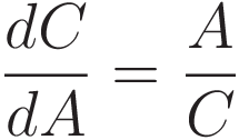
When the length of the side labeled A is changed the length of the hypothenuse C changes with it. For the purpose of deriving Fermat's stationary time we will need an exact expression for the rate of change of the length of line segment C with respect to length change of A.
In the limit of an infinitesimally small increment of the angle the small triangle with sides ΔA and ΔC has the same angles as the triangle with sides C and A. Therefore in the limit of infinitesimally small increment of the angle we have:
To confirm we set up differentiation of C with respect to A, making use of Pythagoras' theorem:
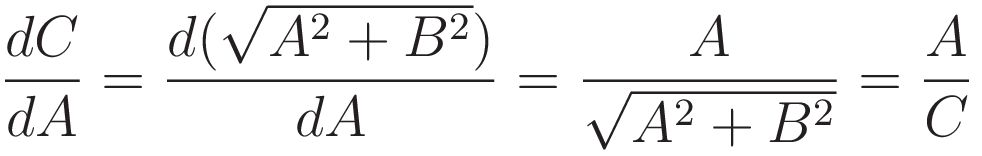
The significance of (4) is this: the ratio A/C is the sine of the angle opposite to A.
This property is key to Fermat's stationary time: the derivative of the length of the hypotenuse with respect to the length of the opposite side is the sine of the opposite angle.
(4) is a geometric property that is not specific to optics or even physics, it is a mathematical property.
In Image 4 the letter 'S' stands for ‘Snell's point’. We will take as our starting point that there is a fixed point from where the light is transmitted, point 'T', and that there is a fixed point 'R' where the light is received. (T and R not shown in the image; T and R can be arbitrarily far away.)
If it is granted that the wavefront is perpendicular to the direction of propagation it follows that the angle β1 is equal to the angle α1, and that the angle β2 is equal to the angle α2.
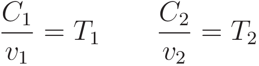
The final piece to be prepared is to state the relation between the length of line C, and the time it takes to traverse that length.
The variation
The variation of the path of the light consists of moving point S along the refraction line. We want to find the criterion that identifies the location of point S in the variation space such that Snell's law is satisfied.
At this point I recommend that you set up two side-by-side instances of your browser, with this page open in both. Use one to read step by step, and use the other to scroll back when the discussion refers to earlier equations.
We start with repeating (3), the relation that follows directly from Huygens wavefront hypothesis.
For the incoming ray and the refracted ray restate the sine as the ratio A/C:
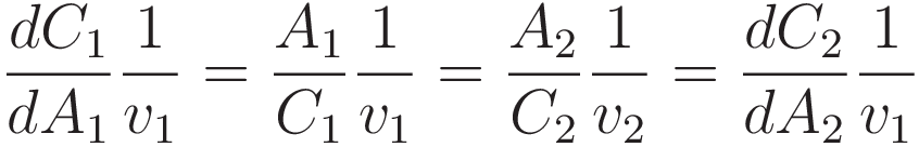
The next step is to make use of (4): dC/dA = A/C, running it in reverse: substitute the ratio A/C with the differentiation operation:
Now that the factor C is in the numerator of the fraction we can absorb the factor 1/v into the differentiation; C/v=T
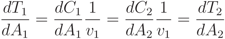
The result:
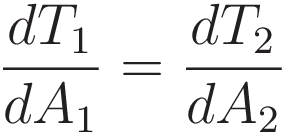
Recapitulating: we started with Huygens wavefront hypothesis, from there obtained Snell's law, and from there we obtained (11).
We have - of course - that A1 and A2 are not independent; increasing A1 by an amount Δ A1 decreases A2 by the same amount; Δ A2 = -Δ A1. Therefore we can restate (11) as derivatives with respect to variation of a single point: Snell's point S. The variation space is a hypothetical space; I will refer to the position in this hypothetical space as Sh.
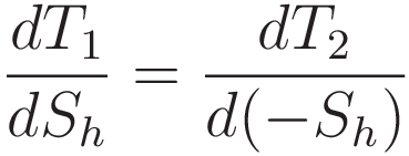
Moving the minus sign outside the differentiation makes it more readable:
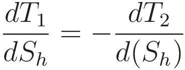
Snell's point is where the derivatives of T1 and T2 have the same magnitude.
Graphlet 5 displays exploration of the hypothetical variation space in accordance with (13). The value displayed in the slider knob is the position of the refraction point Sh in the variation space. We can think of T1 and T2 as functions of the position of point Sh
In the righthand sub-panel: the graph labeled T1 represents the duration for the light to move from the point of emission to the refraction point, the graph labeled T2 represents the duration for the light to move from the refraction point to the point of reception.
Comparing derivatives
The thing that is being evaluated is the derivative of the time. In the variation space: at Snell's point the variation is at a point where the graphs T1 and T2 have the same derivative, with opposite sign. Hence: at Snell's point the variation is at a point where the derivative of the sum (T1 + T2) is zero.
This brings us to Fermat's stationary time. 'Stationary' as in: you are looking for the point in variation space where the derivative of (T1 + T2) is zero.
Discussion
At this point let's look back on what has been established.
Snell's law is formulated in terms of the sines of the angle of incidence and angle of refraction respectively. The significance of that is: for the phenomenon of refraction it is the angle that counts.
The geometric property (4) is what allows Snell's law to be restated in terms of differentials; the derivative of the length of the hypotenuse with respect to the length of the opposing side.
From (8) to (10): dividing by the velocity v changes the spatial lengths (C1,C2) to the durations (T1,T2).
This brings us to (11): although visually (11) looks to be an equation in terms of derivatives, it is still about angles. (11) is equivalent to Snell's law, and Snell's law is about angles.
Multiple paths
Light taking multiple paths from a single start point to a single end point
Diagram 6 shows a setup with a stack of three prisms. This represents the geometry of a Fresnel lens in a schematic way. To see how often Fresnel lenses are used my recommendation is to google with the search terms:
"magnifier" "fresnel lens"
The diagram represents that light emitted from a single start point is refracted onto a single end point. We have for the three paths that for each the total duration is different.
Switching to the wavefront hypothesis: we observe that all of the paths that the light is taking are accounted for in terms of the wavefront hypothesis.
In fact: our general experience is that all the properties of propagation of light can be accounted for in terms of the wavefront hypothesis.
In diagram 6 each of the three paths has the following property: compared to closely adjacent paths the duration of the path is stationary.
Refraction at a curved interface
Refraction of light, curved surface
In graphlet 7 The egg shaped region represents a chunk of glass. For simplicity the index of refraction is assigned a value of 1.5
That is: to traverse 1 unit of distance through the glass takes 1.5 units of time.
The slider changes the radius of the upper circle. The graphlet decreases the radius of the lower circle by the amount such that the sum of the transit times remains 2.5 units of time.
The point of intersection of the two circles traces out a shape that has the property that all the rays that travel from point A to point B have the same transit time.
The radio button 'modify' switches the graphlet to a form such that the user can modify the egg shape.
With an increased curvature of the air-glass interface: the light from point A that reaches point B has traveled the path of most time.
This graphlet is designed for the purpose of demonstrating that Fermat time is not about least time. Instead the criterion is: light travels along a path such that the derivative of the transit time is zero.
That derivative-of-the-transit-time is the derivative with respect to variation. The variation moves the point of refraction along the air-glass interface.
Reflection
Reflection of light in the case of a flat surface
In graphlet 8: the variation space is the length of the straight line where the light will reflect. This particular variation space is a 1-dimensional space. As the slider is moved the exploratory point sweeps out variation. As we know: if we grant Huygens' wavefront hypothesis then it follows that the true reflection point is the point such that the angle of reflection is equal to the angle of incidence.
In the section right-angled triangles a geometric property of the hypotenuse of a right-angled triangle was demonstrated: the derivative of the length of the hypotenuse (with respect to the triangle width) is equal to the sine of the hypotenuse's angle.
(In the case of reflection the velocity of the light is the same along the entire path, therefore using length-of-the-path or duration-of-the-path is equivalent.)
At the true reflection point the angles are equal.
Therefore: the derivatives of the lengths will be equal in magnitude (while being opposite in sign).
Therefore: the derivative of the sum of the lengths will be zero.
In graphlet 8: the number underneath the exploratory reflection point gives the sum of the two lengths. When the exploratory reflection point is at the true reflection point the derivative of the sum of the lengths is zero.
Reflection of light in the case of a concave surface
In graphlet 9 the variation space is the length of the concave surface. The concave surface is in the shape of an ellipse. In the starting configuration the ratio of major axis and minor axis is such that the two focal points of the ellipse coincide with the point of emission and the point of reception. As a consequence: everywhere in the variation space the derivative of the total pathlength (with respect to variation) is zero .
Moving the lower slider modifies the major axis of the ellipse. Decreasing the major axis makes the reflecting surface more concave. With a more concave surface the true reflection point is at a maximum in the variation space.
All of the above combined demonstrates that Fermat's stationary time is not about minimizing time. The criterion is: identify the point in variation space such that the derivative of the time (with respect to variation) is zero.
The total time is not a relevant factor here. The relevant factor is the derivative of the time; taking the derivative of the length of the path recovers the angle.

This work is licensed under a Creative Commons Attribution-ShareAlike 3.0 Unported License.
Last time this page was modified: April 12 2026