Least action visualized
In this article I explore the 'Action' of the 'Principle of least Action'. I discuss how the Principle of Least Action relates to the laws of motion.
About the name 'least action': while that name is (still) very common, it is generally acknowledged that the name 'stationary action' is preferable in the sense that 'stationary action' reflects the nature of the physics in a way that 'least action' does not. Hamilton's stationary action asserts that when the trial trajectory coincides with the true trajectory the derivative of Hamilton's action is zero. There are classes of cases such that when the trial trajectory coincides with the true trajectory Hamilton's action is at a maximum. Hamilton's action can be a minimum or a maximum.
It is always the case, however, that when the trial trajectory coincides with the true trajectory the derivative of Hamilton's action is zero.
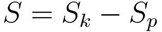
The usual notation for the 'Action' is the letter 'S'. For the Energy I will use the letter 'E', with subscript; 'k' for 'kinetic' and 'p' for 'potential'
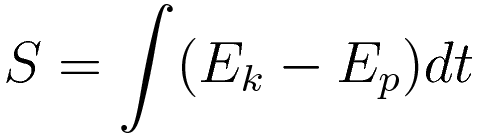
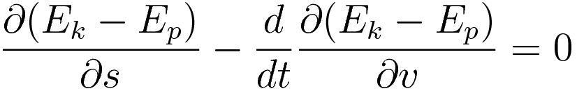
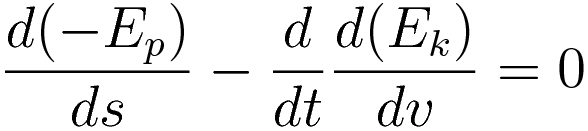
The evaluation of the Action consists of taking the derivative of the Action. We have that when the Action is evaluated for a range of trajectories the derivative of S with respect to the variation is zero for the case of the true trajectory. How is it that the quantity (Ek - Ep) has that property?
Diagrams
As the title indicates: the emphasis is on visualization.
Diagrams 2, 3, 4, and 5 each have a slider; moving the slider sweeps out a range of trial trajectories. From here on I will refer to the diagrams with a slider as 'graphlet' (graphical javascript applet).
Separate evaluation
Instead of subtracting Ep from Ek early on I will evaluate the time integrals of Ek and Ep separately. Combining the two will be postponed until the very last step.
Preparation
Differentiation - Integration
There is a specific property of integration that is key to the nature of the principle of least action
As we know, we use differentation of a curve to find the slope of that curve, and we use integration of a curve to find the area enclosed between that curve and some horizontal line.
Here's the thing: when the slope of a curve changes the value of that curve's integral changes in proportion. Take the simplest case: f(x) = ax Change of the magnitude of the slope changes the value of the integral. This property is key.
For emphasis I repeat in a box section:
Force acting over distance; the work-energy theorem
Here I demonstrate the case of a uniform force, hence uniform acceleration; the result generalizes to a force that is not uniform but dependent on position.
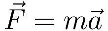
To obtain the work-energy theorem we start with the force-acceleration principle:
The following expressions follow from definitions. Velocity is defined as the time derivative of position; acceleration is defined as the time derivative of velocity. Given those definitions we have the following expressions that every mechanics texbook starts with:
Change of velocity as a function of time:
Change of position as a function of time:
(1.3) and (1.4) are not independent; differentiation of (1.4) gives (1.3). Conversely, (1.4) can be thought of as the result of integration of (1.3)
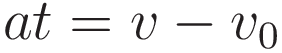
In preparation for later use: rearrange (1.3)
Take (1.4), move s0 to the left hand side, and multiply everything with acceleration a
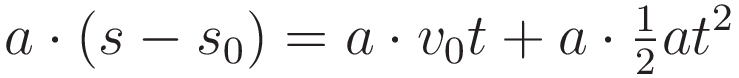
Rearrange to prepare for applying (1.5)
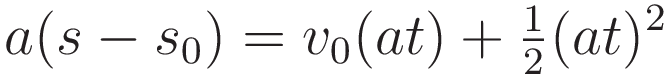
Use (1.5) to substitute (at)

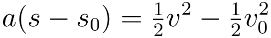
Multiply out the right hand side:

The crossterm vv0 drops out, and we arrive at a remarkably clean result:
If we take the initial position s0 and the initial velocity v0 as zero then (1.10) simplifies to:
(The above expression is also known as Torricelli's formula)
With the above in place we go back to the force-acceleration principle:
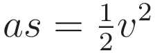
multiply both sides of (1.12) with s, the position coordinate.

Use Torricelli's formula, (1.11), to resolve the right hand side to an expression in terms of v for velocity:
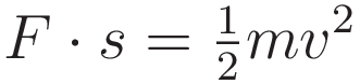
With initial position s0 and the initial velocity v0 not zero it takes the following form

Force acting over a distance (s - s0) is called doing work.
The above was demonstrated for uniform acceleration. For the more general case, with an acceleration that changes over time, the same relation is formulated in terms of an integral: the integral of force acting over distance:
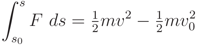
The work-energy theorem is the reason it is meaningful to define potential energy and kinetic energy.
As we know: potential energy is defined as the negative of work done.
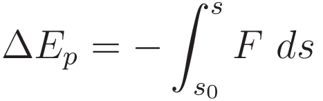
The demonstration in this article is for the classes of cases where the force is a conservative force. When the force is conservative there is a defined potential energy. From this point onward I will be using the expression 'potential energy'.
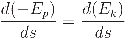
The validity of the Work-Energy extends to arbitrarily small increments of motion. During the entire time the rate of change of kinetic energy must match the rate of change of potential energy.
The setup
An object shoots upward, released to free motion. The object climbs, decelerated by gravity, reaches its highest point, and falls back again.
To work with round numbers I have selected the following conditions:
- Total duration: 2 seconds (from t=-1 to t=1)
- Gravitational acceleration: 2 m/s2
- Mass of the object: 1 unit of mass.
Those conditions imply that along the true trajectory the starting velocity is 2 m/s, and the object climbs to a height of 1 meter.
Diagram 1 gives the height (vertical axis) of the object as a function of time (horizontal axis). The graph representing the motion is of course a parabola. Expression (2.1) gives that parabola.

Class of trial trajectories
Graphlet 2 shows how the trajectory is varied, generating a class of trial trajectories. (In this graphlet, and in the subsequent graphlets, you can slide to other values by dragging the circle with the mouse.) The startpoint and endpoint are fixed, in between the trajectory is varied. The set of all possible variations of the trajectory is much larger than this particular class of course, but for the purpose of this demonstration this simplest case is sufficient.
More generally, the constraint is that the variation must preserve the fixed startpoint and endpoint. Superficially that may not look particularly constraining, but in fact it is. This significant constraint is a key element.
With the trajectory being varied in the way presented in graphlet 2 we need just a factor pv which stands for 'variational parameter'. Now each trajectory is a function of two variables: 't' and 'pv'
In the graphlet, use the slider to see the range of trial trajectories.

As you can see, when the variational parameter pv is zero expression (2.2) simplifies to expression (2.1).
Kinetic energy
To prepare the ground for comparing kinetic and potential energy graphlet 3 shows a trivial case: how the evaluation comes out if there is no force (and therefore no potential energy). Then in the graph the true trajectory is a straight line. The diagram on the left shows a range of trial trajectories, the diagram on the right represents the kinetic energy at each point in time.
As we know: the integral of kinetic energy over time is equal to the size of the shaded area.
Kinetic energy and potential energy
Repeating expression (2.2) for the trajectory as a function of time t and the variational parameter pv.
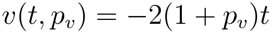
The derivative of function (2.2) with respect to time gives the velocity.
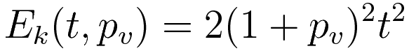
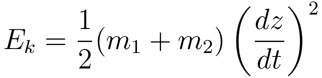
Entering the velocity (2.3) in the formula 1/2mv2 gives expression (2.4) for the kinetic energy. Expression (2.5) is obtained by multiplying the height (2.2) with the gravitational acceleration (which has the value 2 in this example.)

Matching the rate of change of energy
Graphlet 4:
- Red curve: kinetic energy Ek
- Green curve: minus potential energy Ep
- Slider: variational parameter pv
The demand is that at every point along the trajectory the rate of change of kinetic energy must match the rate of change of potential energy
The graphlet uses the minus potential energy because that is what is being compared.
The height at which the potential energy has been placed is arbitrary; as we know potential energy does not have an inherent zero point. For the comparison that makes no difference; what is being compared is the derivative of the kinetic energy and the derivative of the potential energy.
Response to variation
As you sweep out the variation there is only a single value of the variational parameter pv where the slopes of the two curves match. That's because the magnitude of the kinetic energy is a quadratic function of pv and in the case displayed in the diagrams the magnitude of the potential energy is a linear function of pv.
This difference is independent of the way you are sweeping out the variation. Whatever way you implement the variation: as you sweep it out the kinetic energy is more sensitive to it than the potential energy.
This concludes the discussion of the physics of the principle of least action.
The mathematics
From here on I will refer to the 'red curve' and the 'green curve'. Partly because that's just shorter, but mainly to emphasize that this part of the demonstration is about mathematics only.
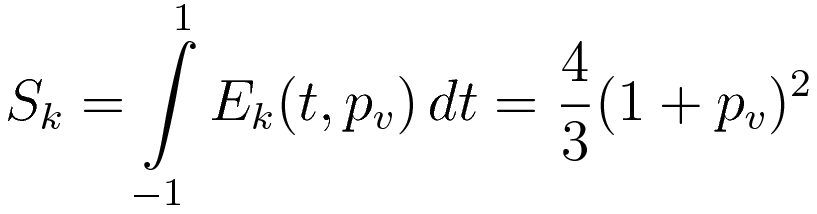
As announced at the start, combining the components of the action is postponed until the very last step. I define the action components Sk (kinetic energy component) and Sp (potential energy component).
The following integrals are integrals over time: from t=-1 to t=1.
The kinetic energy (2.4) evaluates to (3.3)
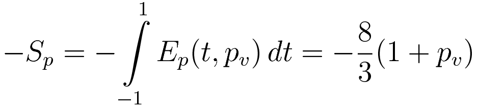
In the case of the potential energy there is the fact that the evaluation compares the kinetic energy with the minus potential energy. To accommodate that I have added minus signs throughout. (2.5) evaluates to (3.4)
For future reference: the total action:
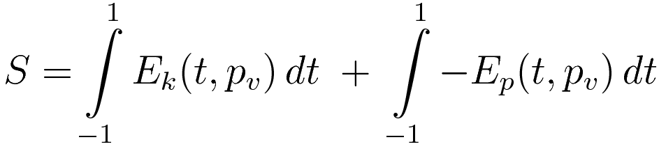
However, the minus sign can be moved inside the integration, and then the total action can be thought of as the sum of two integrals: the integral of the kinetic energy and the integral of the minus potential energy:
Graphs
Graphlet 5 pulls everything together:
The top half is the same as graphlet 4.
The curves in the lower-left quadrant are the same curves as in the upper-right quadrant, but a different property is emphasized: as you vary the trial trajectory the respective slopes of the energy curves change at a different rate.
In this case the response of the curve for the potential energy to trial trajectory variation is linear, since in this case the potential energy itself is a linear function of the height.
The kinetic energy is proportional to the square of the velocity, hence the response of the curve for the kinetic energy to trial trajectory variation is quadratic.
To capitalize on the property emphasized in the lower-left quadrant I turn to the property of integration that I mentioned at the start: when you change the slope of a curve the value of that curve's integral changes in proportion.
The checkbox: blue graph: the sum of the two integrals.
(About the reason why the checkbox in the lower right subpanel says 'sum'. The diagram displays graphs for the kinetic energy and the minus potential energy. The blue line that appears when you check the checkbox gives the result of summing the two graphs.)
(The thing that I believe is actually causing confusion: in our mathematical notation the minus sign is used for two purposes: one is to state a negation, such as minus potential energy, the other is to state an operation: subtraction. That is: when it says: (EK - EP) we should understand that as: (EK + -EP).)
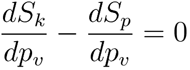
The subdiagram in the lower-right quadrant stands out from the others. The graphs in the lower-right quadrant are functions of the variational parameter pv. Hence the slopes of those graphs correspond to the derivative with respect to pv. When the variation is at the true trajectory the combined derivative evaluates to zero:
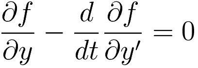
The Euler-Lagrange equation
As we know, the Euler-Lagrange equation is a general variational calculus equation. It facilitates finding an extremum of a functional.
In the case of dynamics the equation of motion you are looking for describes position as a function of time, so here I give the functional S in that form.
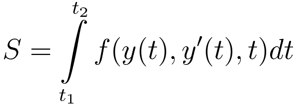
The Euler-Lagrange equation identifies a stationary point of the functional S
In the following I will explain how it is possible that the solution to an equation stated in integral form (integral of the Lagrangian) can be found with an equation that is a differential equation
A key point is this: the fact that you are looking for an extremum (minimum or maximum) is actually a very constraining condition.
I will start with a specific case, and then I will generalize.
Consider expressions (3.3) and (3.4), both are integration from t=-1 to t=1, in notation ∫-11f(t)dt. What if you would cut that up, and compute two adjoining integrals, ∫-10, and ∫01?
For emphasis I'm putting the following property in a box section.
To generalize this: the integration is over a certain timeframe, we can call that: from t1 to t2. You can subdivide that timeframe in subsections. The overall integration will be minimal if and only if the integrals of each of the subsections are minimal. There is no limit to how far you can subdivide, hence this extends to infinitisimally short subsections. This means it must be possible to restate the problem as a differential equation.
(The first to recognize this lemma was Jacob Bernoulli, publishing in 1697. See the appendix 'Jacob's Lemma'. It may well be that this lemma was independently rediscovered multiple times.)
Preetum Nakkiran has devised a derivation that capitalizes on this property: geometric derivation of the Euler-Lagrange equation
Energy mechanics
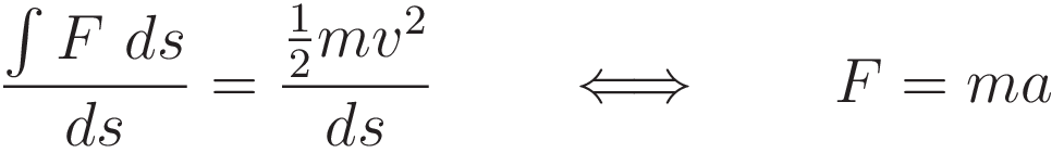
The following expression gives the idea of expressing physics taking place in terms of energy in the most concise way:
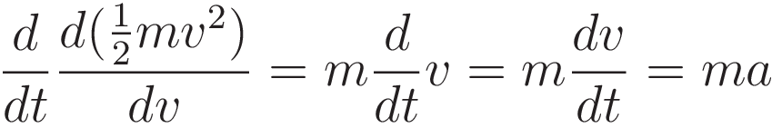
The point is: (5.1) is another way of stating F=ma, since taking the derivative with respect to position recovers F=ma:
The following sequence shows the steps of taking the derivative of the kinetic energy with respect to position:
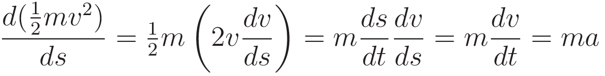
(Here I have used v for 'velocity'. When using generalized coordinates this generalizes to the first derivative of the position in terms of the generalized coordinates.)
Comparison with Euler-Lagrange equation
Before I go further let me first go over the verification that using Lagrangian-in-EL-equation is equivalent to applying the condition that the rate of change of kinetic energy must match the rate of change of potential energy
The Euler-Lagrange equation is a very general equation, more general than is needed for the purpose of classical mechanics. The full EL-equation with the Lagrangian:
For the purpose of this comparison the Lagrangian-in-EL-equation simplifies to the following form:
The term with the potential energy is already identical to the one in the energy equation (5.1).
Evaluating the term with kinetic energy:
(5.3) and (5.6) evaluate to the same expression. This completes the verification that the Lagrangian-in-EulerLagrange-equation (5.4) is identical to the energy equation (5.1).
Example
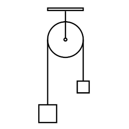
Atwood machine
The Atwood machine is the simplest example of using generalized coordinates.
Of course the purpose of this example isn't to demonstrate the Atwood machine, it's to demonstrate that using generalized coordinates doesn't depend on anything else. Using generalized coordinates isn't tied to any particular formalism. This example demonstrates using equation (6.2)
The two weights move in opposite directions, but since the velocity is squared that is inconsequential. Using the letter z for the amount of displacement:
The kinetic energy:
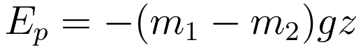
The potential energy:
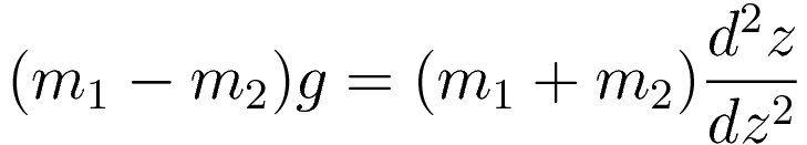
Substituting in the energy equation (6.2) and taking the derivatives:
The efficiency of the energy approach
When the motion has more than one degree of freedom the force-acceleration equation has to be written in vectorial form, and then you have vectorial form both for the force and the acceleration:
That's a redundancy and in computations that redundancy comes with a workload.
In energy mechanics the velocity is squared and thus the directional information of the velocity term is lost. That's an advantage, as all of the directional information is still there, expressed in the gradient of the potential. Now a single term is carrying directional information instead of both; by removing redundancy a more powerful instrument has been created.
The key points
- The mathematical property that identifies the true trajectory is independent of the way the variation is implemented. As you sweep out the variation: the way the kinetic energy is sensitive to it is different from the way the potential energy is sensitive to it.
- Making start point and end point fixed sets up the following property: changing the the slope of the energy curve changes the value of the integral in proportion.
- The demonstration is for a specific case: uniform force. The reasoning generalizes to all cases.
- The foundation of the Euler-Lagrange equation is this: the value of the overall integral is an extremum (minimum/maximum) if and only if the value is minimum/maximum along every subinterval. This extends to infinitisimally short subintervals. This is why the Euler-Lagrange equation is a differential equation.
- The combination of using generalized coordinates and the energy approach is more efficient than the force-acceleration approach.
Appendix I: Jacob's Lemma
There is a lemma in variational calculus, first stated by Jacob Bernoulli. (Therefore I propose to name it 'Jacob's Lemma'.)
When Johann Bernoulli had presented the Brachistochrone problem to the mathematicians of the time Jacob Bernoulli was among the few who solved it. The treatment by Jacob Bernoulli is in the Acta Eruditorum, May 1697, pp. 211-217
Jacob opens his treatment with an observation concerning the fact that the curve that is sought is a minimum.
Jacob's Lemma
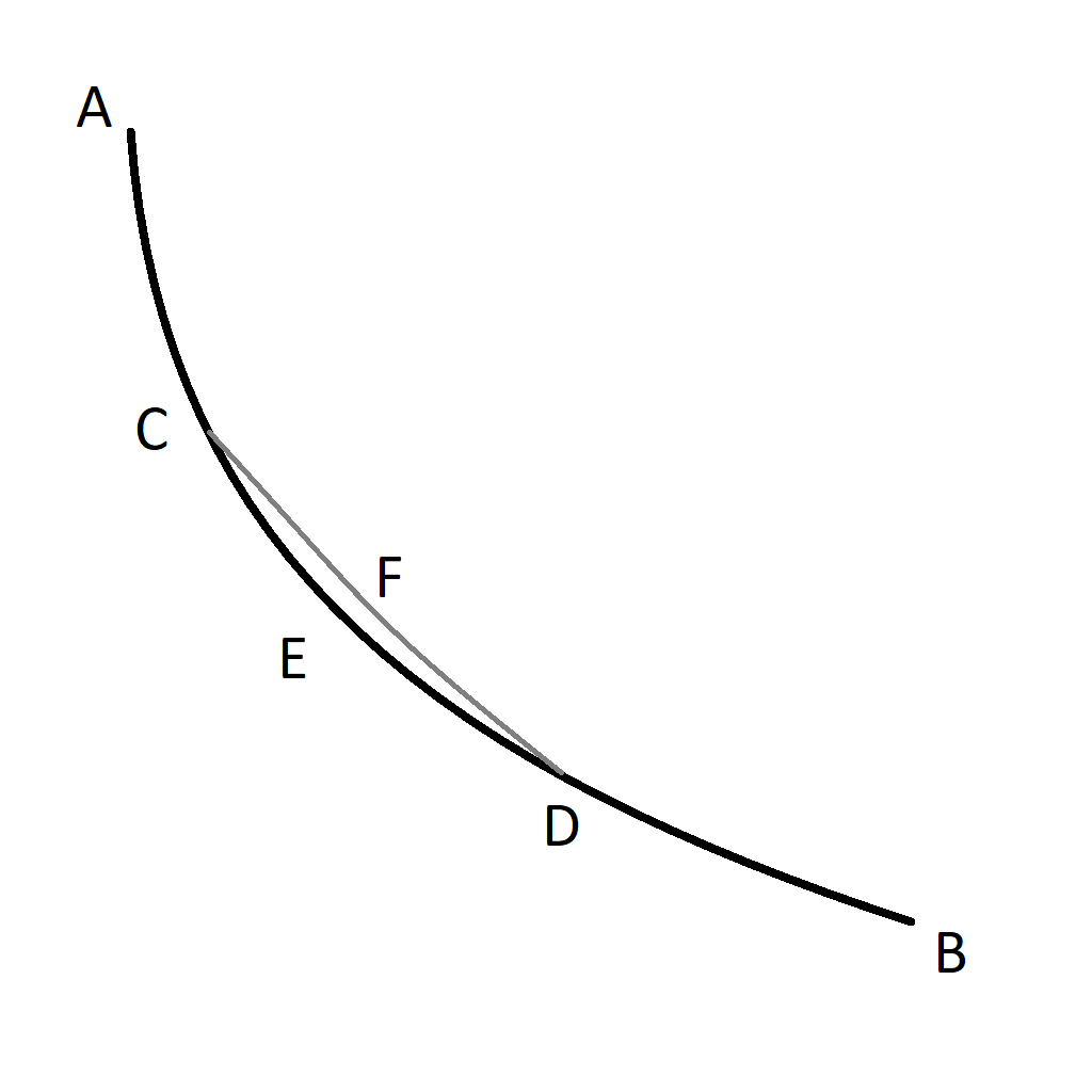
Lemma. Let ACEDB be the desired curve along which a heavy point falls from A to B in the shortest time, and let C and D be two points on it as close together as we like. Then the segment of arc CED is among all segments of arc with C and D as end points the segment that a heavy point falling from A traverses in the shortest time. Indeed, if another segment of arc CFD were traversed in a shorter time, then the point would move along ACFDB in a shorter time than along ACEDB, which is contrary to our supposition.
Appendix II: derivation of the Work-Energy theorem
The derivation in the main article uses Torricelli's formula (1.9). Torricelli's formula is the product of integration in the following sense: if you take the time derivative of (1.6) you get (1.5), which means that (1.6) can be thought of as the result of the integral over time of (1.5).
The following derivation states the integration explicitly. The integration is key to what the Work-Energy theorem is.
The steps in the following derivation are all towards the end goal of obtaining an expression in terms of the velocity v. In the course of the derivation the following two relations will be used:
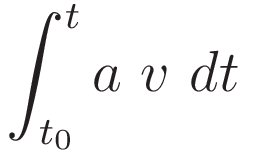
The integral for acceleration from a starting point s0 to a final point s
Intermediary step: change of the differential according to (II.1), with corresponding change of limits.
Change the order:
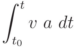
Change of the differential according to (II.2), with corresponding change of limits.
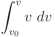
So we have:
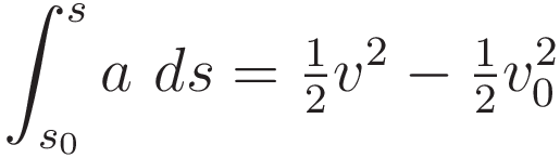
Up to this point no physics has been stated. (II.7) follows from the definitions of velocity and acceleration, combined with the mathematical properties of differentiation/integration.
Multiplying both sides with m and combining with F = ma arrives at a physics statement: the Work-Energy theorem:
The interactive animations on this page were created with the Javascript Library JSXGraph. JSXGraph is developed at the Lehrstuhl für Mathematik und ihre Didaktik, University of Bayreuth, Germany.

This work is licensed under a Creative Commons Attribution-ShareAlike 3.0 Unported License.
Last time this page was modified: January 24 2024