The calculations in the Foucault pendulum simulation

This page accompanies the page with the Foucault pendulum simulation. Here I discuss the way that the calculations have been set up.

The coordinate system is spherical coordinates, with θ (theta) as the counterpart of longitude and φ (phi) as the counterpart of latitude. As everywhere else on this site I use the capital letter Ω to denote the angular velocity of the system as a whole, and I use the small letter ω for the instantaneous velocity of some object. Ω is a constant; it does not change over the course of a simulation run.

In the case of an actual Foucault pendulum the wire's suspension point is above the surface, so that gravity provides the restoring force for the pendulum. In this simulation the restoring force is expressed as an elastic force that acts towards a point of attraction, and this point of attraction is on the surface itself.

Ω	Angular velocity of the rotating system
ψ	the pendulum's oscillation rate
φ_attract	The latitude of the attraction point
φ	Angle (in radians) between equatorial plane and current latitude
ω_φ	Angular velocity parallel to longitude line.
θ	Angular position of the particle
ω	Angular velocity parallel to latitude line

The simulation evaluates the following set of differential equations:

$\begin{cases} \cfrac{d\phi}{dt} & = \; \omega_\phi \\ \cfrac{d\omega_\phi}{dt} & = \; - \sin(\phi)\omega^2 \cos(\phi) \ - \ \psi^2(\phi - \phi_{attract}) \\ \cfrac{d\theta}{dt} & = \; \omega \\ \cfrac{d\omega}{dt} & = \; 2 \sin(\phi) \omega_\phi \, \omega/\! \cos(\phi) \ - \ \psi^2(\theta - \Omega t) \\ \end{cases}$

Because of the algorithm that EJS uses the differential equations must be declared in the above form, with first derivatives but no second derivatives.

I will build up to the above system of equations in three stages:

Inertial motion along a flat surface, in polar coordinates
Inertial motion along the surface of a sphere, in spherical coordianates
Addition of the force that is exerted upon the pendulum bob

Especially, note that the system of equations is for the motion with respect to the inertial coordinate system. Usually Foucault pendulum calculations are set up for motion with respect to the co-rotating coordinate system. However, using equations of motion for the inertial coordinate system has the advantage that the calculation itself offers a clear view of the cause of the pendulum precession. The elastic force towards the point of attraction, in the simulation view represented with the green vector, is the force that is evaluated by the system of equations.

Derivation

Polar coordinates

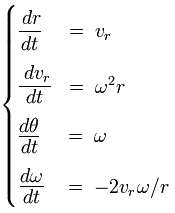
The following system of equations describes inertial motion along a flat surface, in polar coordinates.

r	Radial distance
v_r	Velocity in radial direction.
θ	Angular position of the particle
ω	Angular velocity

$\begin{cases} \cfrac{dr}{dt} & = \; v_r \\ \cfrac{dv_r}{dt} & = \; \omega^2 r \\ \cfrac{d\theta}{dt} & = \; \omega \\ \cfrac{d\omega}{dt} & = \; - 2 v_r \omega/ r \\ \end{cases}$

Inertia

The form of the equations arises from using polar coordinates. The motion is decomposed in perpendicular directions: motion in radial direction and motion in tangential direction. When using polar coordinates the coordinate system gridlines are not straight of course, and inertia gives objects a tendency to move in straight lines, so the inertia must be incorporated explicitly.

The second differential equation, d(v_r)/dt = ω²r , is straightforward. An inward directed force that causes an acceleration of ω²r, sustains uniform circular motion with angular velocity ω. In the absence of such a centripetal force the instantaneous radial acceleration (outward) will be ω²r.

The fourth equation represents conservation of angular momentum.
We have the following expression for angular momentum: L = mωr² . Angular momentum is conserved in two cases: when there is no force at all, and when there is a centripetal force (this is described in the article about conservation of angular momentum). Here the mass m is constant, so the conservation of angular momentum narrows down to conservation of the quantity ωr² .

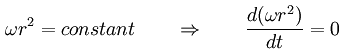
$\omega r^2 = constant \qquad \Rightarrow \qquad \frac{d(\omega r^2)}{dt} = 0$

Differentiating the expression for the angular momentum:

$r^2 \frac{d\omega}{dt} + \omega \frac{d(r^2)}{dt} = 0$

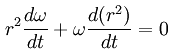
Using the chain rule we obtain an expression in terms of a factor dr/dt .

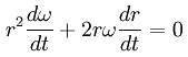
$r^2 \frac{d\omega}{dt} + 2 r \omega \frac{d(r)}{dt} = 0$

Rearranging, dividing left and right by r², and substituting dr/dt with v_r, we obtain the fourth differential equation:

$\cfrac{d\omega}{dt} & = - 2 v_r \omega/ r$

This derivation illustrates the origin of the factor 2 in the equation. The factor 2 is connected with the fact that angular momentum is proportional to the square of the radial distance.

When polar coordinates are used the representation of inertia takes on the form of differential equations. In other words, when polar coordinates are used we find that we have to use expressions typical for dynamics to represent inertia, giving inertia the appeareance of a force. In general, when non-cartesian coordinates are used we get explicit expressions that represent inertia, whereas when cartesian coordinates are used the representation of inertia is implicit.

From polar coordinates to spherical coordinates

Spherical coordinates are for 3 spatial degrees of freedom, but here the radius of the sphere is set to a constant 1. With only 2 spatial degrees of freedom; latitude and longitude, the equations in spherical coordinates for the Foucault pendulum simulation are still for motion along a surface, but this time it's a curved surface rather than a flat surface.

The cosine of the latitude

If the radius of the sphere is R, then the distance r of a particle to the central axis of rotation is given as follows: r = cos(φ)R . With R = 1 we have the following substitution r = cos(φ).

The sine of the latitude

The factor ωr² represents the tendency of a circumnavigating object to swing wide. But away from the poles this tendency is diminished, and on the equator there is obviously no opportunity at all to swing wide. The diminishment of the tendency to swing wide is proportional to the sine of the latitude.

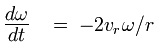
The differential equation dω/dt = 2ωv_r/r must be adjusted too. Only the component of ω_φ that is perpendicular to the central axis of rotation contributes to change of ω. That implies the following substitution: v_r = -sin(φ)ω_φ

In the system of equations for spherical coordinates the sine factor has a minus sign. The reason for that is that the zero point of φ is not at the poles but at the equator. In polar coordinates r is zero at the center and it increases outwardly. In spherical coordinates that is reversed: zero at the equator and towards 90 degrees latitude increasing, hence the minus sign.

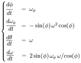
In all this gives us the system of equations for inertial motion over the surface of a sphere. On the left is the system of equations for motion over a flat surface, on the right the equations for motion over the surface of a sphere.

φ	Angle (in radians) between equatorial plane and current latitude
ω_φ	Angular velocity parallel to longitude line.
θ	Angular position of the particle
ω	Angular velocity parallel to latitude line

$\begin{cases} \cfrac{dr}{dt} & = \; v_r \\ \cfrac{dv_r}{dt} & = \; \omega^2 r \\ \cfrac{d\theta}{dt} & = \; \omega \\ \cfrac{d\omega}{dt} & = \; - 2 v_r \omega/ r \\ \end{cases}$

$\begin{cases} \cfrac{d\phi}{dt} & = \; \omega_\phi \\ \cfrac{d\omega_\phi}{dt} & = \; - \sin(\phi)\omega^2 \cos(\phi) \\ \cfrac{d\theta}{dt} & = \; \omega \\ \cfrac{d\omega}{dt} & = \; 2 \sin(\phi) \omega_\phi \, \omega/\! \cos(\phi) \\ \end{cases}$

Simulation

The Inertia on a sphere .zip file contains the .xml file for an EJS simulation that works with the above equations for spherical coordinates. A particle that is set in motion proceeds with uniform velocity along a great circle.

The restoring force

For swing amplitudes that are very small relative to the distance to the central axis of rotation the following expressions are a good approximation for the force that sustains the pendulum oscillation.

Ω	Angular velocity of the rotating system
ψ	the pendulum's oscillation rate
φ_attract	The latitude of the pendulum's suspension point

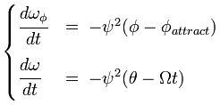
$\begin{cases} \cfrac{d\omega_\phi}{dt} & = \; - \psi^2(\phi - \phi_{attract}) \\ \cfrac{d\omega}{dt} & = \; - \psi^2(\theta - \Omega t) \\ \end{cases}$

The angular velocity parallel to the longitude lines, ω_φ, is an angular velocity with a fixed distance to the origin of the coordinate system. Therefore the distance (along the surface) between the pendulum bob and the attraction point in longitudinal direction is proportional to (φ - φ_attract)

The attraction point is circumnavigating the central axis with angular velocity Ω, so the longitudinal position of the attraction point is given by the expression Ωt. There's a catch: further away from the central axis the quantity (θ - Ωt) corresponds to a larger distance (along the sphere's surface). To get the actual distance the expression must be multiplied with r, the radial distance to the central axis of rotation: (θ - Ωt)r. But the expression must also be divided by r, because the differential equation is for angular acceleration, dω/dt, so the factor r cancels out.

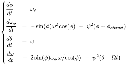
The equations of motion

Adding the expressions for the attracting force to the system of equations for inertial motion over the surface of a sphere gives the system of equations that is evaluated by the Foucault pendulum simulation.

The mass of the pendulum bob

In the above equations pendulum bob's mass is not represented. Interestingly, the bob's mass drops out of the equations completely.

The oscillation rate of a Foucault pendulum is independent from the mass of the pendulum bob. A Foucault pendulum is a gravity pendulum; gravity provides the restoring force. In the equation of motion for a gravity pendulum the bob's mass drops out of the equation because gravitational mass is equivalent to inertial mass.

The equivalence of gravitational and inertial mass is also why the mass drops out of the Foucault pendulum equations of motion entirely. A non-swinging pendulum bob is effectively a plumb line, and a plumb line does not point in the direction of the Earth's center of gravitational attraction. There is an outward displacement, that provides the required centripetal force for co-rotating with the Earth. This outward displacement is the same for any mass, since gravitational mass is equivalent to inertial mass.

Even though the mass drops out the equations are still dynamical equations. There is back and forth conversion of kinetic energy and potential energy; there is exchange of momentum. The precession of the Foucault pendulum is a dynamical process.

This work is licensed under a Creative Commons Attribution-ShareAlike 3.0 Unported License.

Last time this page was modified: June 18 2017