The Foucault pendulum - part 2

The equation of motion that was derived in part 1 of this article is as follows:

$\begin{cases} \dfrac{d^2x}{dt^2} = - \psi^2 x + 2 \Omega \dfrac{dy}{dt} sin(\phi) \\ \dfrac{d^2y}{dt^2} = - \psi^2 y - 2 \Omega \dfrac{dx}{dt} sin(\phi) \end{cases}$

The solution to the equation of motion involves sines and cosines, so to avoid confusion I replace the factor sin(φ) with a single letter. sin(φ) = f. In meteorology the letter 'f' is the usual notation for factoring in the sine of the latitude. Specifically: in meteorology 2Ωsin(φ) = f. It may well be that the letter 'f' was chosen with Foucault in mind.

Using complex number notation, the system of two equations can be restated as a single equation.

$\bigg(\dfrac{d^2x}{dt^2} + i\dfrac{d^2y}{dt^2} \bigg) + 2 \Omega i \bigg( \dfrac{dx}{dt} + i\dfrac{dy}{dt} \bigg) f + \psi^2 \bigg( x + iy \bigg) = 0$

When Ω is much smaller than ψ the following is a good approximative solution to the equation of motion.

$x + iy =e^{-i f \Omega t}\left(c_1 e^{i\psi t}+c_2 e^{-i\psi t}\right)$

The relation e^iφ = sin(φ) + icos(φ) allows the solution to be notated in a compact form. c₁ and c₂ are constants that are determined by the initial conditions, and 'f' is the sine of the latitude.

Picture 1. Image
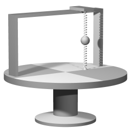
A Wheatstone pendulum setup with the attachment points aligned with the central axis of rotation.

Picture 2. Image
Wheatstone's device

In the case where the angular velocity Ω of the rotating system is zero the expression simplifies to the part inside the parentheses:

$c_1 e^{i\psi t}+c_2 e^{-i\psi t$

Image 1 shows a version of the Wheatstone pendulum where the bob is some distance away from the center, but the suspension points are aligned with the central axis of rotation. When the bob is vibrating, and the device as a whole is rotating then the motion with with respect to the rotating system is described by the full solution:

$x + iy =e^{-i f \Omega t}\left(c_1 e^{i\psi t}+c_2 e^{-i\psi t}\right)$

The factor 'f' equals one in this case, which means that with respect to the rotating system the plane of swing will turn with angular velocity Ω. If the rotating systems rotates counterclockwise with angular velocity Ω then the plane of swing turns clockwise with angular velocity Ω. As seen from an inertial point of view the plane of swing remains pointing in the same direction. It's important to be aware that this preservation of direction is not due to inertia in the sense of Newton's first law. Rather, the preservation of the direction reflects a symmetry of harmonic force. The centripetal force that sustains the circumnavigation is a harmonic force, and motion under its influence possesses remarkable symmetries.

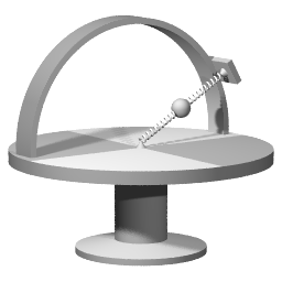
In the case of the setup depicted in image 2 the factor f is 0.5, and completing a full cycle of the vibration will take two full cycles of the rotating system.

The Eötvös effect

One of the simplifying assumptions has been that the weight of the pendulum bob remains exactly the same. In fact the effective weight is affected by the pendulum motion. This is the Eötvös effect, which in the case of a Foucault pendulum gives rise to an asymmetry. There will be a small difference in the pendulum frequencies for the NS and EW directions. The mathematical treatment of this effect can be found on Joe Wolfe's Foucault pendulum discussion, in the section about various complications.

Spherical geometry, parallel transport and anholonomy

Picture 3. Image
Parallel transport along sections of geodesics. Moving along a geodesic of the sphere's surface (a section of a great circle) the vector's angle with respect to the great circle is kept constant.
Image source: Wikipedia

Picture 4. Animation
A Foucault pendulum located at 30 degrees latitude takes two sidereal days to complete a precession cycle.

There have been several authors who have pointed out that there is an isomorphy between the sine law of the pendulum precession and the sine law that arises in the case of parallel transport of a vector over the surface of a sphere.

Parallel transport

Image 3 shows parallel transport along a loop consisting of three sections that follow a great circle, with the three section meeting at right angles. The sum of the angles at each corner equals the total difference in angle when the loop is closed. In the general case the amount of sections can be taken arbitrarily large and in the limit of infinitisimally short sections any smooth loop can be traced.

Sine factor

Picture 5. Image
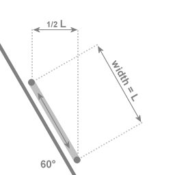
In the case of an angle of 60 degrees with the central axis of rotation: If the two extremal points of the swing are a distance of L apart, then the motion towards and away from the central axis covers a distance of 1/2 L

What the Foucault pendulum and the parallal transport approach have in common is the sine factor. In the case of the Foucault pendulum the sine factor arises in the way that is illustrated with Image 5. In the case of the anholonomy when a vector is parallel transported along a latitude line the sine factor arises from the geometry.

The parallel transport wheel

Picture 6. Animation
Platform and wheel. The wheel can swivel freely. When the platform sets into motion the wheel is forced to follow, but there is no torque to make the wheel rotate around its axis.

Picture 7. Animation
The wheel's support is rigidly attached, the wheel can swivel freely with respect to its support. When the platform sets into motion some rotation is imparted to the wheel.

Animations 6 and 7 present analogues of the Foucault effect.

I will refer to the large disc as 'the platform' and to four spokes with spheres attached as 'the wheel'. The trivial case is not depicted; when the wheel is at right angles to the platform then when the platform sets into motion the orientation of the wheel relative to the platform will remain the same; the platform can exert the torque on the wheel to make it rotate around an axis that is parallel to the platform's axis.

With the setup as depicted in animation 6 there is no opportunity to exert a torque on the wheel.

The setup depicted in animation 7 is an intermediate case: with an angle corresponding to 30 degrees latitude half the torque is exerted, hence the rotation rate that is imparted to the wheel is half the rotation rate of the platform.

In the case of the setups depicted in animations 6 and 7 the wheel does not have to be located near the rim of the disc. The same effect will occur when the center of mass of the wheel coincides with the platform's axis of rotation.

I refer to the setup depicted in animations 6 and 7 as 'the parallel transport wheel' because the way that the orientation of the wheel changes in response to being put in motion is described by parallel transport of a vector over the surface of a sphere.

Both in the case of the Foucault pendulum and in the case of the parallel transport wheel inertia is involved, but not in the same way. To illustrate the difference it is interesting to describe the observation that triggered Foucault in to considering the Foucault pendulum. Foucault had clamped a stiff rodd in a lathe, and he twanged the rod, probably getting a vibration with a deflection of a centimeter or so. When Foucault turned the chuck of the lathe by hand he noticed that the orientation of the rod's plane of vibration remained the same. Evidently it's necessary to distinguish between the actual material of the rod, and the immaterial plane of vibration. It's the immaterial plane of vibration that is locked onto a particular orientation in space. To change that orientation a torque must be exerted.

When Foucault had noticed the behavior of the rod's vibration as the rod co-rotated with the chuck, it occurred to him that the same would apply in the case of a large pendulum on either of the Earth's poles. The wire and the bob will rotate with respect to the immaterial plane of swing, but that is inconsequential. That reduces the demands on the pendulum suspension. The suspension must be perfectly symmetrical, it should not favor any direction of swing, but there is no need to mechanically compensate for the Earth's rotation (comparable to the mechanism for telescopes to compensate for the Earth's rotation.)

In the case of a non-polar Foucault pendulum: before its launch the bob is already circumnavigating the Earth's axis. What is set up with the pendulum launch is a particular direction in space of the immaterial plane of swing. After the launch the constraints acting upon the pendulum bob rotate the direction of the immaterial plane of swing.

Parallel transport references

John B. Hart, Raymond Miller, Robert L. Mills, A simple geometric mode for visualizing the motion of a Foucault pendulum American Journal of physics 55(1), January 1987
John Oprea Geometry and the Foucault Pendulum The American Mathematical Monthly, Vol. 102, No. 6 (Jun. - Jul., 1995), pp. 515-522
Jens von Bergmann and HsingChi A. Wang, Foucault Pendulum through basic Geometry (PDF-file, 209 KB) (submitted for publication in 2005)

This work is licensed under a Creative Commons Attribution-ShareAlike 3.0 Unported License.

Last time this page was modified: July 10 2022