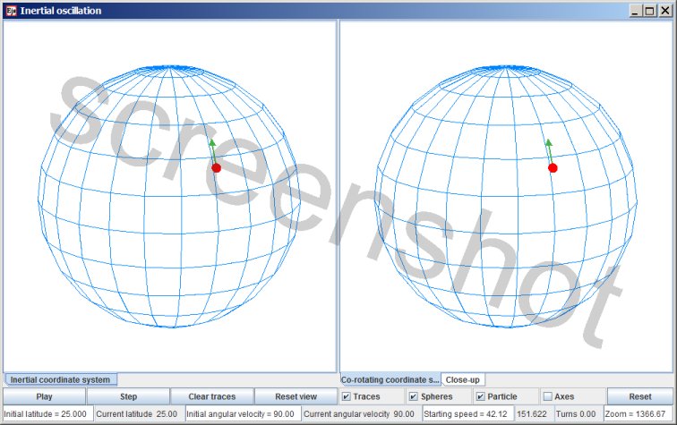
Inertial oscillation
Blue arrow: gravity, acting towards the center of gravitational attraction
Red arrow: normal force, such as the buoyancy force acting on a ship.
Green arrow: the poleward force; the resultant force of gravity and the normal force.
For the atmosphere, which experiences hardly any friction, the poleward force provides the required centripetal force.
The simulation shows the motion of a particle that is moving over the surface of an oblate spheroid. The spheroid is flattened to an ellipsoid of revolution because it is rotating, just as the Earth is flattened because it is rotating. The particle is confined to motion along the surface by the spheroid's gravity; the motion parallel to the surface is treated as frictionless. The green arrow represents a force that arises from the non-sphericity of the ellipsoid of revolution.
Downhill slope
The Earth's equator is about 20 kilometes further away from the Earth's center than the poles are. This means that the Equator is higher ground; from the equator to the poles is a downhill slope. At 45 degrees latitude the slope is a 1/10th of a degree. Let's say you have a hovercraft weighing 10 000 kilogram. On a 1/10th of a degree slope that gives a force of 175 kilogram.
For objects that can slide over the Earth's surface with no friction the following applies: at every latitude the fact that the Earth's surface constitutes a downhill slope provides the centripetal force that is required to remain co-rotating with the Earth at a fixed latitude. In the simulation that centripetal force is represented with the green arrow. I will refer to this centripetal force as the poleward force.
Evolution of the simulation
When the simulation opens the initial latitude is set to 25 degrees, and the initial angular velocity is set to 90; 90% of the angular velocity for co-rotating with the Earth. So at the start the particle is circumnavigating the Earth's axis slower than the Earth itself; the particle is outpaced by the Earth. The amount of centripetal force that the particle experiences at its latitude is the amount that sustains co-rotating motion, hence the particle is subject to a surplus of centripetal force. The surplus pulls the circumnavigating particle closer to the central axis of rotation and in the process the particle gains angular velocity. By the time the angular velocity has increased to 100 (100 % of co-rotating velocity) the particle has acquired an inward velocity. Moving yet closer to the central axis of rotation the particle's angular velocity increases some more, topping at circumnavigating 11 % faster than the Earth's rotation rate. (The angular velocity reaches the value 111.) Circumnavigating the central axis faster than the Earth itself there is not enough centripetal force to sustain that, and the particle swings wide, acquiring a velocity away from the central axis. Moving away from the central axis the particle's angular velocity decreases, and after it has overshot the equilibrium latitude once more the particle is circumnavigating slower than the rotation rate of the Earth, at which point there is a surplus of centripetal force again.
As it happens the default setting of initial latitude 25 degrees and initial angular velocity 90% results in a trajectory that loops back on itself, but that is exceptional. The vast majority of settings results in non-closing trajectories.
The default setting of the simulation shows an extremely exaggerated size of the inertial oscillation. In the case of actual inertial oscillations of bodies of ocean water the total motion is in the order of several kilometers back and forth, which corresponds to less than the width of a pixel on the screen.
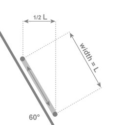
In the case of an angle of 60 degrees with the central axis of rotation: If the two extremal points of the oscillation are a distance of L apart, then the motion towards and away from the central axis covers a distance of 1/2 L
The period of the inertial oscillation is dependent on the latitude. Close to the poles the period of the inertial oscillation is close to 12 hours; there are nearly 2 oscillations per day. See the Coriolis effect physlet to see the reason for this 2:1 ratio. Around 30 degrees latitude there is one inertial oscillation cycle for every period of the Earth. The closer to the Equator the longer the period of the inertial oscillation.
Image 2 illustrates why at lower latitudes the period of the inertial oscillation is longer. For example, at 30 degrees latitude the motion towards and away from the central axis of rotation is reduced, and the change of angular velocity of the oscillating mass is proportional to the motion towards and away from the central axis of rotation.
The westward drift of the motion with respect to the Earth is called the Beta effect (often notated with the greek character: the β-effect) Closer to the equator the trajectory curves less strong than at higher latitudes, so overall the trajectory with respect to the Earth will not be a closed loop. The smaller the size of the inertial oscillation the weaker the β-effect.
The simulation's controls
Initial latitude. The value in this field is in degrees. If you move the object very close to the equator (by setting the Initial latitude to a small value, for example 10) then the arrow representing the poleward force is very small; close to the equator the component of the centripetal force in the direction parallel to the local surface is small.
Initial angular velocity. The value in this field is a percentage; the percentage of co-rotating motion. 100% is co-rotating with the Earth. For input the field only accepts values between 0 and 100.
Starting speed. The value in this field is velocity in westward direction relative to the Earth. Zero is co-rotating with the Earth. For input the fields accepts velocities that corresponds to values of 'Initial angular velocity' that are between 0 and 100%.
A physically realistic velocity for a body of water mass in a state of inertial oscillation is 0.2 meter per second.
Zoom. The simulation adjusts the zoom level in advance to fit the programmed inertial oscillation. The number in the zoom field corresponds to the amplitude of the inertial oscillation in kilometers. A physically realistic inertial oscillation has an amplitude in the order of several kilometers.
When you start altering a value in an input field the field turns yellow. As long as the field is still yellow the input process is not ready. The input is finalized by pressing the Enter key on the keyboard, and then the field will no longer be yellow.
Meteorology and Oceanography
In Oceanography inertial oscillation is recognized as a wide-spread phenomenon, and the physical mechanism that is behind this rotation-of-Earth phenomenon is referred to as the Coriolis effect.
As shown in the introduction of the inertial oscillation article, when there are persistent winds a large mass of water will get some velocity relative to the Earth. When the winds subside that mass of water will continue in an inertial oscillation.
The effect simulated here is central to meteorology, and to the science of ocean currents. Whenever a body of air mass or water mass has a velocity relative to the Earth its motion relative to the Earth tends to deflect to the side. On the northern hemisphere to the right, and on the southern hemisphere to the left. For all directions of velocity relative to the Earth, west, north, east or south, the tendency to deflect to the side is the same.
When a force is present, such as pressure gradient force, the resulting acceleration relative to the Earth will be the vector sum of the Coriolis effect influence and the pressure gradient force influence. The interplay of Coriolis effect and pressure gradient force is discussed in the article about formation of cyclonic flow
Other simulations
A 3D simulation (Java applet) that presents a rotation-of-Earth-effect that I refer to as 'centrifugal effect': great circles.
The 2D interactive animation Coriolis effect.
Method of computation
I discuss the mathematical setup of the inertial oscillation simulation in a separate article: Inertial oscillation mathematics.
In the computations for this simulation the left panel, the inertial point of view, is the primary panel. The equations of the simulation are the motion equations for the motion with respect to the inertial coordinate system.
The trajectory depicted in the right panel is a derivative depiction; it is derived from the trajectory depicted in the left panel, using coordinate transformation.
Download options
This simulation has been created with EJS
EJS stores the specifications of a simulation in a plain text file, with extension .xml
You can examine how the simulation has been set up by opening the simulation .xml file with EJS.
Download location for the EJS software
Download location for the inertial oscillation source file
(The file is zipped because a browser will attempt to parse any .xml file.)
Back to the article in which the physics of inertial oscillation is discussed extensively.
EJS is licenced under a GNU GPL license .

This work is licensed under a Creative Commons Attribution-ShareAlike 3.0 Unported License.
Last time this page was modified: June 18 2017