Great circles - motion over the surface of a rotating sphere
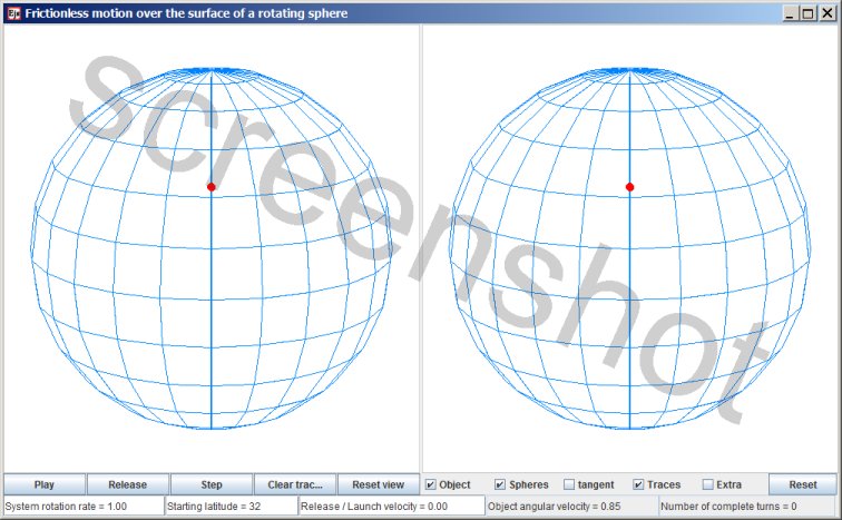
The red dot represents a particle that can slide frictionless over the surface of a perfect sphere. The particle cannot leave the surface. The view on the left represents the motion as seen from an inertial point of view. The view on the right represents the co-rotating point of view, so that the motion relative to the rotating sphere is clearly seen.
If you think of the sphere as a planet, with the planet's gravity confining the object to motion along the surface, then the simulation is physically unrealistic in the following way: a rotating planet always has an equatorial bulge. A rotating planet with a perfectly spherical shape would violate the laws of physics; rotation always induces a bulge. (Of course, this applies only for celestial bodies that are large enough to self-gravitate to an equilibrium shape. Very small celestial bodies, such as asteroids, do not have enough self-gravitation to affect their own shape.)
In this simulation the sphere is indeed perfectly spherical, and there is no friction, therefore the sphere does not influence the particle's direction of motion over its surface. Whether the sphere is rotating underneath the particle or not makes no difference for the motion of the object; there's no dynamics going on; there is no exchange of momentum, no change of kinetic energy.
Evolution of the simulation
When the simulation is started with the Play button then initially the particle is located on the starting latitude, co-rotating with the sphere (which of course implies that some retaining mechanism is holding on to the particle). When you press the 'Release' button the particle is released . (The checkbox 'Extra' opens a small panel with additional settings. If the 'Automatic release' checkbox is checked then if not released manually the particle will be released automatically after a full rotation has been completed). Once released the particle proceeds to move along the great circle that is tangent to the starting latitude. Moving along a great circle is the equivalent of moving along a straight line. On a sphere the shortest distance between two points is a (section of) a great circle, just as on a flat surface the shortest distance between two points is a straight line.
Uncheck the checkbox 'Spheres': then you get an unobstructed view of the trajectories. You can manipulate the image with the mouse, turning and pitching the view. You can see then that the motion along the great circle is always tangent to the starting latitude.
The simulation's controls
There are four input fields: 'System rotation rate', 'Starting latitude', 'Release/launch velocity' and 'Object angular velocity'.
- System rotation rate. (1) Inputting a larger value speeds up the evolution, and inputting a smaller value slows down the simulation's evolution. (2) Inputting zero as 'System rotation rate' makes the simulation behave differently. Then the motion relative to the sphere is the same in both panels, so you can compare with the case of a rotating sphere.
The direction of the system rotation, if non-zero, is always counterclockwise (as seen from above). If you input a negative value then that minus sign will be ignored. - Starting latitude. The latitude is measured in degrees.
- Release/launch velocity. This value is not expressed in units of velocity; it's a percentage. At each latitude it is the percentage of the velocity for co-rotating with the sphere at that latitude. You can input any positive or negative value for the Release/launch velocity. The smoothest release is when you input a value of zero, then it is a release. A non-zero value is a change of velocity for the particle, so that is a launch.
- Object angular velocity. For the angular velocity of the particle as it moves along a great circle. 'System rotation rate' and 'Object angular velocity' are scaled the same, so if you input the value '1' for the Object angular velocity then the particle will complete a great circle in one full rotation of the system.
General remark: if you input a new value for any of the above four input values then one or more of the other inputs will be updated to keep those four input values in an overall consistent state.
When you start altering a value in an input field the field turns yellow. As long as the field is still yellow the input process is not ready. The input is finalized by pressing the Enter key on the keyboard, and then the field will no longer be yellow.
Purpose
The reason I designed this simulation is that I wanted to create a vivid illustration of what happens when the particle is launched with a velocity in westward direction.
Set 'System rotation rate' to zero. Then both when launched to the left and when launched to the right the particle proceeds to the equator, moving along a great circle. Check the checkbox 'Tangent' to get the tangent great circle. Following the tangent great circle is what you expect for the non-rotating setup. Set 'System rotation rate' to 1 again, and input a moderate westward launch, such as -10 or -20. You will see that the object deflects to the left of the tangent circle.
Centrifugal effect
I refer to the rotation effect that is illustrated with this simulation as centrifugal effect. The comparison is between what happens in the case of a non-rotating sphere and in the case of a rotating sphere. An object is launched with moderate velocity relative to the sphere.
In the case of a non-rotating sphere:
- A launched object, launched either to the East or to the West, proceeds towards the equator. The motion relative to the sphere will follow a great circle. (Check the box 'Tangent' so see the tangent great circle.)
- Initially co-rotating with the sphere, the particle has a velocity to begin with; the launch with moderate velocity either increases or decreases that initial velocity. The motion follows a great circle, but as the sphere rotates underneath the particle the motion relative to the sphere will not be along a great circle.
- A particle launched to the East will proceed to the equator faster than in the case of a non-rotating sphere; deviation to the right.
- An object launched to the West will also proceed to the equator, following a trajectory that deviates to the left of the tangent great circle.
Of course, if you launch with extreme velocity things work out a little differently. The checkbox 'Extra' opens a small window with extra settings, including a section with presets. Choose the preset 'Westward launch'. That will set up a starting latitude of 32 degrees, and a release/launch velocity of -47 (minus 47). Then the object will move along the tangent great circle for quite a stretch. With that particular combination of factors the motion relative to the Sphere comes out very similar to the case of a non-rotating sphere. (The release/launch velocity is a percentage. At 32 degrees latitude, a velocity of 47% of the velocity of co-rotating motion is about the speed of sound.)
The case with the least motion towards the equator is when the release/launch velocity is -100, then the object is stopped in its tracks. With an even larger release/launch velocity the object once again will proceed to the equator after launch.
Line of sight
Note that a great circle is also the line of sight. The shortest distance between two points (on a sphere) is a section of a great circle. Reset the view of the simulation and check the checkbox for the tangent circle. The red dot is at the point where the tangent circle is tangent to a latitude line. Something that you are aiming for that is on that tangent circle will be exactly due West in your line of sight.
Relevance for ballistics
A projectile that is expelled by a gun is during it's flight effectively in orbit around the Earth. (But since there is a lot of air resistence the motion of a projectile is generally not referred to as orbital motion.) An orbit is planar, with the Earth's center of mass in the orbital plane, so the line of intersection of the orbital plane and the Earth's surface will be a great circle. This means that this motion-along-a-great circle simulation can serve as a first approximation of projectile motion.
Is the great circles simulation relevant for ballistics? Well, generally other factors, which in one form or another are all air resistance factors, are much larger than the rotation-of-Earth-effect. The rotation-of-Earth-effect is going to be swamped anyway, so you can spare yourself the trouble. But if you do want to take the rotation-of-Earth-effect into account, for instance if you want to work out whether a bolt from a crossbow will be affected, then this simulation shows that you need know to when to correct for a deviation to the left and when to correct for a deviation to the right; it can be either way.
Not applicable in Meteorology
The rotation-of-Earth-effect that illustrated with this simulation is distinct from the rotation-of-Earth effect that is taken into account in Meteorology. The effect that is relevant for Meteorology is represented with the following applet: inertial oscillation.
Method of computation
The trajectory of the object is calculated by separately calculating the x, y, and z-component of the trajectory. The motion is along a great circle, with uniform velocity. So all three components, x,y and z are sine functions, and calculating the motion is simply a matter of evaluating the sine functions. The left panel, the inertial point of view, is the primary panel In the computations. First the motion as depicted in the inertial point of view is calculated. The next step is to transform the trajectory as computed for the left panel to the coordinate system that is co-rotating with the sphere.
Download options
This simulation has been created with EJS
EJS stores the specifications of a simulation in a plain text file, with extension .xml
You can examine how the simulation has been set up by opening the simulation .xml file with EJS.
Download location for the EJS software
Download location for the great circles source file
(The file is zipped because a browser will attempt to parse any .xml file.)

This work is licensed under a Creative Commons Attribution-ShareAlike 3.0 Unported License.
Last time this page was modified: December 26 2019