Ballistics and the Earth's rotation
The simulation is designed to compute ballistic trajectories that range from tens of meters long to kilometers long.
This simulation complements the Ballistics and Orbits simulation. In the case of the ballistics and orbits simulation values for the rotation rate and gravitational acceleration (g) are not preset to match the circumstances on Earth. They are set to values that give a vivid display. This simulation however, uses the actual Earth rotation rate, and the actual gravitational acceleration. The simulation is designed to show the motion as it proceeds in real-time.
When the released object reaches the Earth's surface the simulation halts automatically
This simulation represents the pure ballistics that would occur in the absence of any atmosphere. But in the range of velocities and altitudes involved here air resistence effects are very significant, so the outcomes will not reflect what will happen on Earth.
Also, effects arising from the Earth's equatorial bulge aren't incorporated. The calculations work with a perfect sphere.
The graphics
The diagram on the left
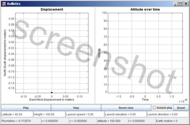
The diagram called 'Displacement' displays a plot of the position of the projectile relative to the point of origin. It doesn't show height, the other diagram does that. The scaling of the x-axis and y-axis is fixed in a 1:1 ratio.
When a simulation is running the line that is drawn traces the motion of the falling object relative to a horizontal plane (as if that horizontal plane is falling together with the object). The two dots in the diagram offer supporting information. The black dot shows the point on the Earth's surface where a plumb line points to. That is, if the object is released from 100 meters high, then the black dot shows where a 100 meter long plumbline will point to. The grey dot shows the position of the plumbline at the current altitude of the falling object. The falling object will always land east of the point where the plumbline points to, but in north-south direction there is hardly any deviation.
The diagram on the right
The diagram called 'Altitude over time' is always a shape that is very close to a parabola. The x- and y-axis scaling are independent, so you need to read the scaling carefully.
Scaling
During the simulation run you will often see on-the-fly rescaling. The diagrams rescale to keep the plot within the diagram's frame. When a simulation run has completed the diagrams jump to a best fit of the plots. At that point you can click the button 'Reset view' and start that simulation run again. This time there won't be any rescaling, as the plots will fit perfectly.
The input fields
- Latitude The latitude, in degrees, from where the projectile is released.
- Height The height, in meters, above the surface of the Earth of the point of release.
- projectile speed How fast the projectile is shot. If you want to simulate dropping an object from, say, a tower, then you release with zero speed. If you want to shoot straight up then obviously there must be a starting speed.
- Launch Elevation Angle, in degrees, with respect to the local surface of the launch.
- Launch direction Angle, in degrees, of the launch direction. Eastward is zero, westward is 180.
When you start to edit an input value the input field turns yellow. To confirm an edit you press the 'Enter' key on the keyboard; the yellow goes away then.
The output fields
- x The East-West position of the projectile, relative to the point where the projectile was released
- y The North-South position of the projectile, relative to the point where the projectile was released
- Altitude The current height above the Earth surface
- t Time counting from the moment the simulation run was started
- Earth motion During the flight of the projectile the Earth is turning underneath it. This value gives how much the point of origin has been moved by the Earth's rotation.
In this simulation all lengths are in meters. 'Height' is in meters, 'Launch speed' is in meters per second, x' is in meters 'y' is in meters, 'Altitude' is in meters, 'Earth motion' is in meters
Compensating for North-South error
For a launch with initial velocity it's to some extent possible to compensate for the fact that the computation works with a perfect sphere rather than with the reference ellipsoid. You calculate the angle of a plumb line at the latitude from which you launch, and then you adjust the value of the 'Launch elevation' accordingly. For example, at 45 degrees latitude you set 'Launch direction' to '90', and 'Launch elevation' to 89.9 Then an object will land very close to the latitude it was launched from.
Method of computation
The method of computation is numerical analysis: the trajectory of the particle is computed by evaluating differential equations.
First the differential equations are used to calculate the motion with respect to the inertial coordinate, subsequently a coordinate transformation is used to transform the trajectory to motion with respect to the co-rotating coordinate system.
This simulation has been created with EJS
EJS stores the specifications of a simulation in a plain text file, with extension .xml
You can examine how the simulation has been set up by opening the simulation .xml file with EJS.
Download location for the EJS software
Download location for the ballistics and orbits source file
(The file is zipped because a browser will attempt to parse any .xml file.)

This work is licensed under a Creative Commons Attribution-ShareAlike 3.0 Unported License.
Last time this page was modified: June 18 2017