Calculus of Variations, Hamilton's stationary action
The main feature of this webpage is the stationary action diagram
The soap film image and the diagram below it are here to provide context.
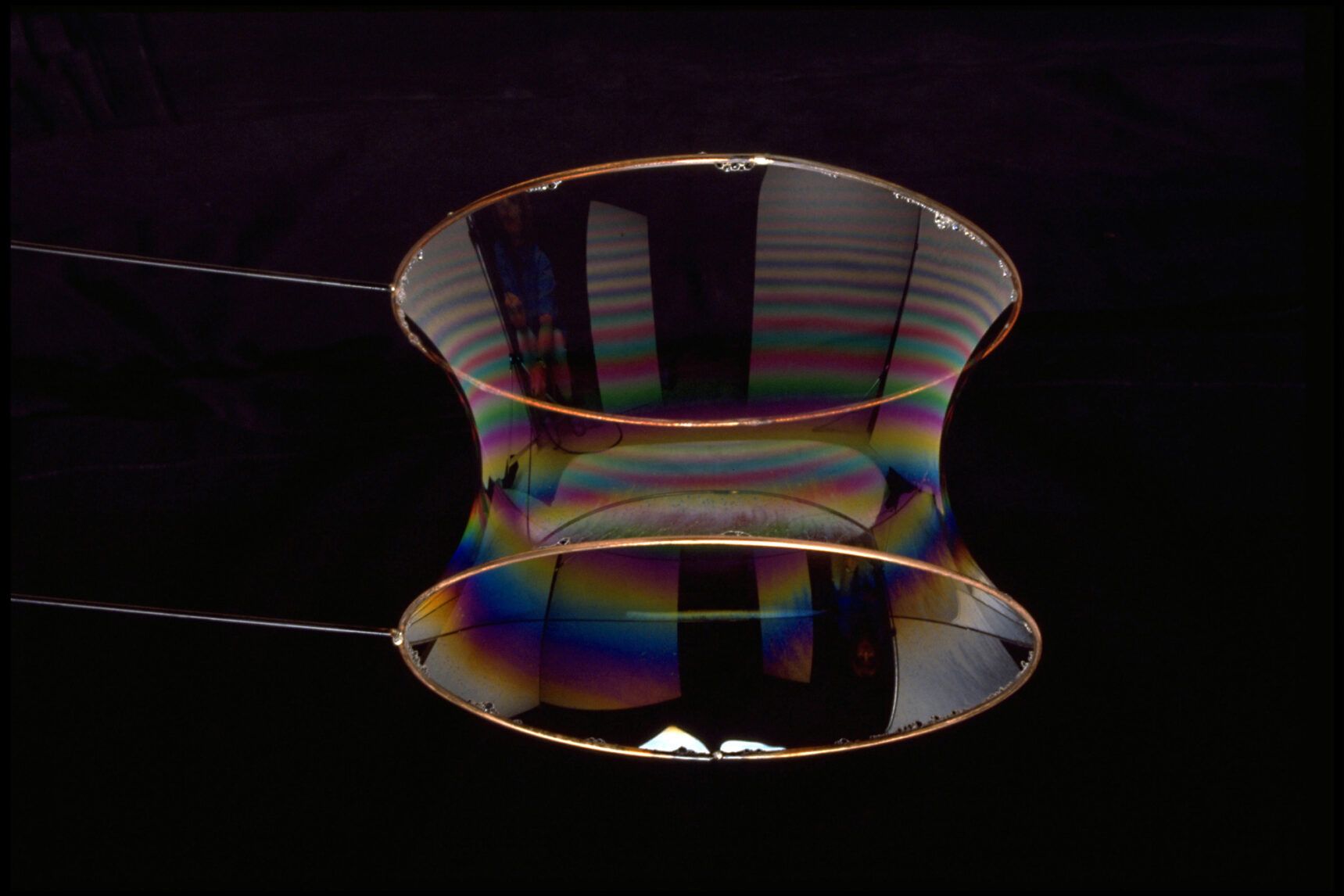
Image credit: Susan Schwartzenberg - Exploratorium
The right hand side of the diagram shows a catenoid surface in cross section. The number in the bottom right corner is the total surface area. Scramble the sliders, and then keep working the sliders to home in on minimized surface area. (To save time, scramble only the first three sliders; leave the fourth in de default position.)
In the final position: for every slider the response to variation is stationary. If on every subsection the response to variation is stationary then for the overall domain the response is stationary.
Calculus of variations is that you take the limit of going to infinitesimally small subsections.
Mathematical implementation of the process expressed in the diagram is described in the article Calculus of Variations, as applied in Physics.
For the next diagram, the main feature, I suggest that you open two side-by-side instances of your browser, with this page open in both instances. Use one of them to scroll through the description so that you're not scrolling up and down all the time.
Potential propertional to the cube of the height
The case represented in the interactive diagram below is the case of an object thrown vertically upward, subject to a force such that the potential increases with the cube of the height.
Of course, a case with a potential that increases with the cube of the height is unlikely to actually occur. The reason for implementing that potential function: the diagram that it produces is particularly well suited to exposition of Hamilton's stationary action.
The interactive display as a whole consists of three subpanels with a sequence of diagrams.
First diagram: the axes are labeled 'time' and 'height'
Second diagram: the axes are labeled 'time' and 'energy'
Third diagram: the axes are labeled 'variation' and 'integral'
The slider sweeps out variation; moving the slider changes the height of the trial trajectory. The display in the second diagram follows the state in the first diagram; the response in the third diagram follows the state in the second diagram.
First diagram
The grey curve is a plot of the true trajectory. The true trajectory was obtained by applying numerical integration, using Runge Kutta 4. With \(h\) for 'height': the magnitude of the acceleration was obtained by differentiating the potential energy with respect to position coordinate: \(\tfrac{d(h^3)}{dh}=3h^2\). In the diagram: at time coordinate \({t=1}\) the object has fallen back all the way to height zero; being back at height zero at \({t=1}\) was achieved by tweaking the initial velocity.
The dashed line is a polynomial approximation of the true trajectory. The polynomial is of the form \({f(x)=a + bx^2+cx^4+dx^6}\). The variation is applied by multiplying the value of the polynomial with the slider value.
In the code that runs the diagram: to obtain the velocity (for the value of the kinetic energy) the polynomial is differentiated with respect to time.
Second diagram
As we know: the sum of kinetic energy and potential energy is a conserved quantity. It follows: for the true trajectory the kinetic energy and the minus potential energy are parallel to each other everywhere along the timeline. That is the reason why in the diagram the potential energy is represented as minus potential energy.
The shape of the energy curve is determined by the following two factors: the shape of the trajectory, and how the energy is a function of the trajectory. As you move the variation parameter slider: it is only at the value 1.00 that the red curve (\(E_k\)) and the green curve (-\(E_p\)) are parallel to each other everywhere along the timeline.
Third diagram
The red dot and the green dot display the value of the respective integrals as function of the variational parameter 'p'. The displayed value is obtained by numerical integration of the curve in the second diagram.
The last step was to fit the colored line (a function of the parameter 'p') such that it tracks the vertical position of the dot.
The diagram demonstrates: as you apply variation: because \({\small \tfrac{1}{2}}mv^2\) is quadratic the response of the kinetic-energy-integral to variation is a quadratic function. For the potential energy: in the case displayed here the potential energy is a cubic function of height; it follows that the response of the potential-energy-integral to variation is a cubic function
The pattern as it plays out in this diagram generalizes to all instances of application of Hamilton's stationary action:
The response of the kinetic-energy-integral is in all cases quadratic because \({\small \tfrac{1}{2}}mv^2\) is a quadratic expression. For the response of the potential-energy-integral: we have that the potential can be any power of the position coordinate. If the potential is to the power \(n\) then response of the potential-energy-integral will be to the power \(n\). Example: for an inverse square law the potential is inversely proportional to radial distance: \(r^{-1}\) Then the response to variation is an \(r^{-1}\) function .
Variation and position coordinate
A key aspect of calculus of variations: the direction of sweeping out the variation coincides with the direction of the position coordinate.
(In this diagram there is one degree of freedom, the relation generalizes to cases with multiple degrees of freedom. With two spatial degrees of freedom: for each of the degrees of freedom a corresponding variation is applied.)
The response of the integral to variation
In the third diagram: as you move the slider you are traversing variation space. At \({p=1.0}\) the derivative of the blue curve is zero. Mathematically, since the blue curve is the sum of the red curve and the green curve: at \({p=1.0}\) the red curve and the green curve have the same tangent angle, with opposite sign.
In the first diagram the cubic nature of the potential determines the shape of the true trajectory. That cubic nature propagates to the integral that is displayed in the third diagram.
The true trajectory has the property that the rate of change of kinetic energy matches the rate of change of potential energy. That property propagates to the respective integrals; the true trajectory has the property that the derivative wrt position of the kinetic-energy-integral matches the derivative wrt position of the potential-energy-integral
Mathematical implementation of the process expressed in the diagram is described in the article about Hamilton's stationary action
Appendix:
How the true trajectory was approximated with a polynomial
This is the structure of the polynomial:
\( \begin{array}{l} - 0.982 (1+t)(-1+t) \\ + 0.400 (1+t) t^2 (-1+t) \\ - 0.150 (1+t)(0.5+t) t^2(-0.5+t)(-1+t) \end{array} \)
The term on the first row sets up an inverted parabola. The top of that parabola sets the polynome at the height of the true trajectory, but everywhere else the curve is too high.
The term on the second row brings the sides down. I opted to set up the second row polynomial in such a way that at x=-0.5 and x=0.5 the sum of the first row term and second row term coincide with the true trajectory.
The third row term brings the sum of all three rows remarkably close to the true trajectory.
To explore what each of the three terms does: use the 'zero' button to set all three to zero, and then explore the individual effect of each slider.
To obtain the value of the kinetic energy we need the derivative with respect to time. To facilitate differentiation of the polynomial the expressions are processed to the following state:
\( \begin{array}{l} - 0.982 (t^2 - 1) \\ + 0.400 (t^4 - t^2) \\ - 0.150 (t^6 - 1.25 t^4 + 0.25 t^2) \end{array} \)

This work is licensed under a Creative Commons Attribution-ShareAlike 3.0 Unported License.
Last time this page was modified: November 01 2025